Introduction
The geometric distribution is used to model situations where we are interested in finding the probability of number of failures before first success or number of trials (attempts) to get first success in a sequence of independent Bernoulli trials, each with probability of success $p$.
There are two different definitions of geometric distributions: one based on number of failures before first success and another based on number of trials to get first success. The choice of definition depends on the context.
Geometric Distribution
Consider a series of mutually independent Bernoulli trials with constant probability of success $p$ and probability of failure $q =1-p$.
Let random variable $X$ denote the number of failures before first success. Then the random variable $X$ takes the values $x=0,1,2,\ldots$.
For getting $x$ failures before first success, we require $(x+1)$ Bernoulli trials with outcomes $FF\cdots (x \text{ times}) S$.
$$ \begin{eqnarray*} P(\text{$x$ failures and then success}& = & P(FF\cdots (x \text{ times})S)\\ P(X=x) & = & q\cdot q\cdots \text{ ($x$ times) } \cdot p\\ & = & q^x p,\quad x=0,1,2\ldots\\ & & \quad 0<p<1, q=1-p. \end{eqnarray*} $$
The name geometric distribution comes from the fact that various probabilities for $x=0,1,2,\cdots$ are the terms from a geometric progression.
Definition of Geometric Distribution
A discrete random variable $X$ is said to have geometric distribution with parameter $p$ if its probability mass function is given by
$$ \begin{equation*} P(X=x) =\left\{ \begin{array}{ll} q^x p, & \hbox{$x=0,1,2,\ldots$} \\ & \hbox{$0<p<1$, $q=1-p$} \\ 0, & \hbox{Otherwise.} \end{array} \right. \end{equation*} $$
Clearly, $P(X=x)\geq 0$ for all $x$ and
$$ \begin{eqnarray*} \sum_{x=0}^\infty pq^x &=& p\sum_{x=0}^\infty q^x \\ &=& p(1-q)^{-1} \\ &=& p\cdot p^{-1}=1. \end{eqnarray*} $$
Hence $P(X=x)$ is a legitimate probability mass function.
Key Features of Geometric Distribution
- A random experiment consists of repeated trials.
- Each trial has two possible outcomes: success and failure.
- The probability of success ($p$) is constant for each trial.
- The trials are independent of each other.
- The random variable $X$ is the number of failures before getting first success $(X = 0,1,2,\cdots)$ OR the number of trials to get first success $(X = 1,2,\cdots)$.
Distribution Function
The distribution function of geometric distribution is $F(x)=1-q^{x+1}, x=0,1,2,\cdots$.
Proof
The distribution function of geometric random variable is given by
$$ \begin{aligned} F(x)&=P(X\leq x)\\ &=1- P(X> x)\\ &=1-\sum_{x=x+1}^\infty pq^x\\ &=1-p(q^{x+1}+q^{x+2}+q^{x+3}+\cdots)\\ &=1-pq^{x+1}(1+q^{1}+q^{2}+\cdots)\\ &=1-pq^{x+1}(1-q)^{-1}\\ &=1-pq^{x+1}p^{-1}\\ &=1-q^{x+1}, x=0,1,2,\cdots \end{aligned} $$
Alternative Form of Geometric Distribution
Sometimes a geometric random variable is defined as the number of trials (attempts) until the first success, including the trial on which the success occurs. In such situations, the p.m.f. of geometric random variable $X$ is given by
$$ \begin{equation*} P(X=x) =\left\{ \begin{array}{ll} q^{x-1} p, & \hbox{$x=1,2,\ldots$} \\ & \hbox{$0<p<1$, $q=1-p$} \\ 0, & \hbox{Otherwise.} \end{array} \right. \end{equation*} $$
The mean for this form is $E(X) = \dfrac{1}{p}$ and variance is $\mu_2 = \dfrac{q}{p^2}$.
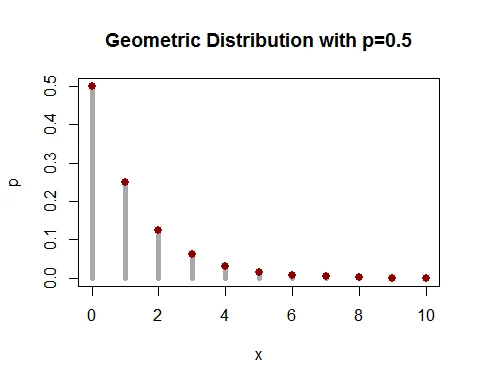
Graph of Geometric Distribution
Following graph shows the probability mass function of geometric distribution with parameter $p=0.5$.
Mean of Geometric Distribution
The mean of geometric distribution is $E(X)=\dfrac{q}{p}$.
Proof
The mean of geometric random variable $X$ is given by
$$ \begin{eqnarray*} \mu_1^\prime =E(X) &=& \sum_{x=0}^\infty x\cdot P(X=x) \\ &=& \sum_{x=0}^\infty x\cdot pq^x \\ &=& pq \sum_{x=1}^\infty x\cdot q^{x-1} \\ &=& pq(1-q)^{-2}\\ &=& \frac{q}{p}. \end{eqnarray*} $$
Variance of Geometric Distribution
The variance of geometric distribution is $V(X)=\dfrac{q}{p^2}$.
Proof
The variance of geometric random variable $X$ is given by
$$ \begin{equation*} V(X) = E(X^2) - [E(X)]^2. \end{equation*} $$
Let us find the expected value of $X^2$.
$$ \begin{eqnarray*} E(X^2) & = & E[X(X-1)+X]\\ &=& E[X(X-1)] +E(X)\\ &=&\sum_{x=1}^\infty x(x-1) P(X=x) +\frac{q}{p}\\ &=& \sum_{x=2}^\infty x(x-1)pq^x +\frac{q}{p}\\ &=& pq^2 \sum_{x=2}^\infty x(x-1)q^{x-2}+\frac{q}{p}\\ &=& 2pq^2 (1-q)^{-3}+\frac{q}{p}\\ &=& \frac{2q^2}{p^2} +\frac{q}{p}. \end{eqnarray*} $$
Now,
$$ \begin{eqnarray*} V(X) &=& E(X^2)-[E(X)]^2 \\ &=& \frac{2q^2}{p^2}+\frac{q}{p}-\frac{q^2}{p^2}\\ &=& \frac{q^2}{p^2}+\frac{q}{p}\\ &=&\frac{q}{p^2}. \end{eqnarray*} $$
Note: For geometric distribution, variance > mean.
Moment Generating Function
The moment generating function of geometric distribution is $M_X(t) = p(1-qe^t)^{-1}$.
Proof
$$ \begin{eqnarray*} M_X(t) &=& E(e^{tX})\\ &=& \sum_{x=0}^\infty e^{tx} P(X=x) \\ &=& \sum_{x=0}^\infty e^{tx} q^x p\\ &=& p\sum_{x=0}^\infty (qe^{t})^x\\ &=& p(1-qe^t)^{-1}. \end{eqnarray*} $$
Mean and Variance from MGF
The mean and variance of geometric distribution can be obtained using the moment generating function:
$$ \begin{eqnarray*} \text{Mean }=\mu_1^\prime &=& \bigg[\frac{d}{dt} M_X(t)\bigg]_{t=0}\\ &=& \bigg[\frac{d}{dt} p(1-qe^t)^{-1}\bigg]_{t=0} \\ &=& \big[pqe^t(1-qe^t)^{-2}\big]_{t=0} \\ &=& pq(1-q)^{-2}=\frac{q}{p}. \end{eqnarray*} $$
Cumulant Generating Function
The cumulant generating function of geometric distribution is $K_{X}(t)=\log_e \bigg(\dfrac{p}{1-qe^t}\bigg)$.
Characteristics Function
The characteristics function of geometric distribution is $\phi_X(t)=p(1-qe^{it})^{-1}$.
Proof
The characteristics function of geometric distribution is
$$ \begin{eqnarray*} \phi_X(t) &=& E(e^{itX})\\ &=& \sum_{x=0}^\infty e^{itx} P(X=x) \\ &=& \sum_{x=0}^\infty e^{itx} q^x p \\ &=& p\sum_{x=0}^\infty (qe^{it})^x\\ &=& p(1-qe^{it})^{-1}. \end{eqnarray*} $$
Probability Generating Function
The probability generating function of geometric distribution is $P_X(t)=p(1-qt)^{-1}$.
Proof
The probability generating function is
$$ \begin{eqnarray*} P_X(t) &=& E(t^{X})\\ &=& \sum_{x=0}^\infty t^{x} P(X=x) \\ &=& \sum_{x=0}^\infty t^{x} q^x p\\ &=& p\sum_{x=0}^\infty (qt)^x\\ &=& p(1-qt)^{-1}. \end{eqnarray*} $$
Lack of Memory Property
Geometric distribution is the only discrete distribution that possesses the lack of memory property.
Suppose a system can fail only at discrete points of time $0,1,2,\cdots$. The conditional probability that a system of age $m$ will survive at least $n$ additional units of time equals the probability that it will survive more than $n$ units of time:
$$ P(X\geq m+n | X\geq m) = P(X\geq n) $$
Recurrence Relation for Probabilities
The recurrence relation to calculate probabilities of geometric distribution is
$$ \begin{equation*} P(X=x+1) = q\cdot P(X=x). \end{equation*} $$
Geometric Distribution Examples
Example 1: Optical Alignment
The probability of a successful optical alignment in the assembly of an optical data storage product is 0.8. Compute the probability that the first successful alignment:
a. requires exactly four trials b. requires at most three trials c. requires at least three trials
Solution
Let $X$ denote the number of trials required for the first successful optical alignment. The probability of success is $p=0.8$, so $q=0.2$.
The probability mass function is:
$$ \begin{aligned} P(X=x)&= p(1-p)^{x-1}; \; x=1,2,\cdots\\ &= 0.8 (0.2)^{x-1}\; x=1,2,\cdots \end{aligned} $$
a. Exactly 4 trials:
$$ \begin{aligned} P(X=4)&= 0.8(0.2)^{4 -1}\\ &= 0.8(0.008)\\ &= 0.0064 \end{aligned} $$
b. At most 3 trials:
$$ \begin{aligned} P(X\leq 3)&= \sum_{x=1}^{3}P(X=x)\\ &= P(X=1)+P(X=2)+P(X=3)\\ &= 0.8+0.16+0.032\\ &= 0.992 \end{aligned} $$
c. At least 3 trials:
$$ \begin{aligned} P(X\geq 3)&= 1-P(X\leq 2)\\ &= 1- \sum_{x=1}^{2}P(X=x)\\ &= 1-\big(0.8+0.16\big)\\ &= 1-0.96\\ &= 0.04 \end{aligned} $$
Example 2: Lighting a Pilot Light
An old gas water heater has a pilot light that must be lit manually. The probability of successfully lighting it on any given attempt is 82%.
a. Compute the probability that it takes no more than 4 tries to light the pilot light. b. Compute the probability that the pilot light is lit on the 5th try. c. Compute the probability that it takes more than four tries.
Solution
Let $X$ denote the number of attempts to light the pilot light. Given $p=0.82$, so $q=0.18$.
The probability mass function is:
$$ \begin{aligned} P(X=x)&= 0.82 (0.18)^{x-1}\; x=1,2,\cdots \end{aligned} $$
a. No more than 4 tries:
$$ \begin{aligned} P(X\leq 4)&= F(4)\\ &=1-q^{4}\\ &=1- 0.18^{4}\\ &=1-0.001\\ &=0.999 \end{aligned} $$
b. On the 5th try:
$$ \begin{aligned} P(X=5)&= 0.82(0.18)^{5 -1}\\ &= 0.82(0.001)\\ &= 0.0009 \end{aligned} $$
c. More than four tries:
$$ \begin{aligned} P(X> 4)&= 1-P(X\leq 4)\\ &= 1- 0.999\\ &= 0.001 \end{aligned} $$
Properties Summary Table
| Property | Formula |
|---|---|
| PMF | $P(X=x) = q^x p$ |
| Mean | $E(X) = \frac{q}{p}$ |
| Variance | $V(X) = \frac{q}{p^2}$ |
| Standard Deviation | $\sigma = \sqrt{\frac{q}{p^2}}$ |
| MGF | $M_X(t) = p(1-qe^t)^{-1}$ |
| Distribution Function | $F(x) = 1-q^{x+1}$ |
| Mode | $x = 0$ (always) |
When to Use Geometric Distribution
The geometric distribution is appropriate when:
- Modeling the number of trials until the first success
- All trials have the same probability of success
- Trials are independent
- We’re interested in the waiting time for a first occurrence
Common Applications:
- Number of attempts until a defective item is found in quality control
- Number of attempts to successfully complete a task
- Number of customer interactions until a sale is made
- Number of experiments until the first successful result
- Reliability testing until first failure occurs
- Number of trials in clinical experiments until first positive response
Conclusion
The geometric distribution is fundamental for modeling waiting times for the first success in repeated independent trials. Its unique lack of memory property makes it particularly valuable in reliability engineering and survival analysis applications.