Simple linear regression from raw data
Let $(x_i, y_i), i=1,2, \cdots , n$ be $n$ pairs of observations.
The simple linear regression model of $Y$ on $X$ is
$$y_i=\beta_0 + \beta_1x_i +e_i$$ where,
- $y$ is a dependent variable,
- $x$ is an independent variable,
- $\beta_0$ is an intercept,
- $\beta_1$ is the slope,
- $e$ is the error term.
Formula
By the method of least square, the model parameters $\beta_0$ and $\beta_1$ can be estimated as
The regression coefficients $\beta_0$ (intercept) and $\beta_1$ (slope) can be estimated as
$\hat{\beta}_1 = \frac{n \sum xy - (\sum x)(\sum y)}{n(\sum x^2) -(\sum x)^2}$
$\hat{\beta}_0=\overline{y}-\hat{\beta}_1\overline{x}$
where,
$\overline{x}=\dfrac{1}{n}\sum_{i=1}^n x_i$is the sample mean of $X$,$\overline{y}=\dfrac{1}{n}\sum_{i=1}^n y_i$is the sample mean of $Y$,- $n$ is the number of data points.
Example
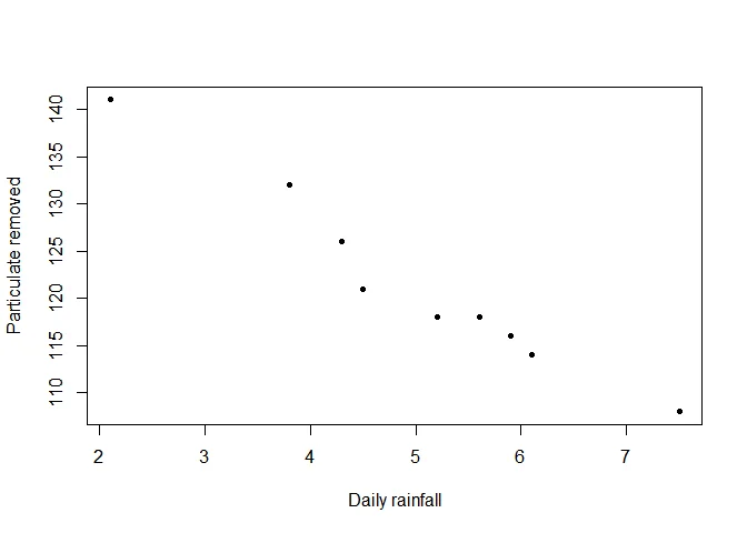
A study of the amount of rainfall and the quantity of air pollution removed produced the following data:
| Daily Rainfall (0.01cm) | 4.3 | 4.5 | 5.9 | 5.6 | 6.1 | 5.2 | 3.8 | 2.1 | 7.5 |
|---|---|---|---|---|---|---|---|---|---|
| Particulate Removed ($\mu g/m^3$) | 126 | 121 | 116 | 118 | 114 | 118 | 132 | 141 | 108 |
a. Find the equation of the regression line to predict the particulate removed from the amount of daily rainfall.
b. Estimate the amount of particulate removed when the daily rainfall is $x=4.8$ units
Solution
Let $x$ denote the daily rainfall and $y$ denote the particulate removed.
Let the simple linear regression model of $Y$ on $X$ is
$$y=\beta_0 + \beta_1x +e$$
By the method of least square, the estimates of $\beta_1$ and $\beta_0$ are respectively
$$ \begin{aligned} \hat{\beta}_1 & = \frac{n \sum xy - (\sum x)(\sum y)}{n(\sum x^2) -(\sum x)^2} \end{aligned} $$
and
$$ \begin{aligned} \hat{\beta}_0&=\overline{y}-\hat{\beta}_1\overline{x} \end{aligned} $$
| $x$ | $y$ | $x^2$ | $y^2$ | $xy$ | |
|---|---|---|---|---|---|
| 1 | 4.3 | 126 | 18.49 | 15876 | 541.8 |
| 2 | 4.5 | 121 | 20.25 | 14641 | 544.5 |
| 3 | 5.9 | 116 | 34.81 | 13456 | 684.4 |
| 4 | 5.6 | 118 | 31.36 | 13924 | 660.8 |
| 5 | 6.1 | 114 | 37.21 | 12996 | 695.4 |
| 6 | 5.2 | 118 | 27.04 | 13924 | 613.6 |
| 7 | 3.8 | 132 | 14.44 | 17424 | 501.6 |
| 8 | 2.1 | 141 | 4.41 | 19881 | 296.1 |
| 9 | 7.5 | 108 | 56.25 | 11664 | 810.0 |
| Total | 45.0 | 1094 | 244.26 | 133786 | 5348.2 |
The sample mean of $x$ is
$$ \begin{aligned} \overline{x}&=\frac{1}{n} \sum_{i=1}^n x_i\\ &=\frac{45}{9}\\ &=5 \end{aligned} $$
The sample mean of $y$ is
$$ \begin{aligned} \overline{y}&=\frac{1}{n} \sum_{i=1}^n y_i\\ &=\frac{1094}{9}\\ &=121.5556 \end{aligned} $$
The estimate of $\beta_1$ is given by
$$ \begin{aligned} b_1 & = \frac{n \sum xy - (\sum x)(\sum y)}{n(\sum x^2) -(\sum x)^2}\\ & = \frac{9*5348.2-(45)(1094)}{9*(244.26)-(45)^2}\\ &= \frac{-1096.2}{173.34}\\ &= -6.324. \end{aligned} $$
The estimate of intercept is
$$ \begin{aligned} b_0&=\overline{y}-b_1\overline{x}\\ &=121.5556-(-6.324)*5\\ &=153.1756. \end{aligned} $$
The best fitted simple linear regression model to predict particulate removed from daily rainfall is
$$ \begin{aligned} \hat{y} &= 153.1756+ (-6.324)*x \end{aligned} $$
The estimate of the amount particulate removed when the daily rainfall is $4.8$ (0.01 cm) is
$$ \begin{aligned} \hat{y}&=153.1756 + (-6.324)\times 4.8\\ &= 122.8204\quad \mu g/m^3 \end{aligned} $$
Computation of various sum of squares
| $x$ | $y$ | $\hat{y}$ | $(y-\hat{y})^2$ | $(\hat{y}-\overline{y})^2$ | $(y-\overline{y})^2$ | |
|---|---|---|---|---|---|---|
| 1 | 4.3 | 126 | 125.9823 | 0.0003 | 19.5961 | 19.7531 |
| 2 | 4.5 | 121 | 124.7175 | 13.8198 | 9.9979 | 0.3086 |
| 3 | 5.9 | 116 | 115.8640 | 0.0185 | 32.3938 | 30.8642 |
| 4 | 5.6 | 118 | 117.7612 | 0.0570 | 14.3971 | 12.6420 |
| 5 | 6.1 | 114 | 114.5992 | 0.3590 | 48.3909 | 57.0864 |
| 6 | 5.2 | 118 | 120.2908 | 5.2478 | 1.5996 | 12.6420 |
| 7 | 3.8 | 132 | 129.1443 | 8.1550 | 57.5890 | 109.0864 |
| 8 | 2.1 | 141 | 139.8951 | 1.2208 | 336.3389 | 378.0864 |
| 9 | 7.5 | 108 | 105.7456 | 5.0823 | 249.9547 | 183.7531 |
| Total | 45.0 | 1094 | 33.9605 | 770.2580 | 804.2222 | 45.0000 |
- Explained variation
$$ \begin{aligned} SSR &= \sum(\hat{y}-\overline{y})^2\\ &=770.258 \end{aligned} $$
- Unexplained variation
$$ \begin{aligned} SSE &= \sum (y-\hat{y})^2\\ &=33.9605 \end{aligned} $$
- Total variation
$$ \begin{aligned} SST &= \sum (y-\overline{y})^2\\ &=804.2222 \end{aligned} $$
- Coefficient of determination
$$ \begin{aligned} R^2 &=\frac{SSR}{SST}\\ &= \frac{770.258}{804.2222}\\ &=0.9578 \end{aligned} $$
$95.78$ percent of the variation in dependent variable is explained by the independent variable.
- Standard error of estimate
$$ \begin{aligned} S_e &= \sqrt{\frac{\sum(y-\hat{y})^2}{n-2}}\\ &=\sqrt{\frac{SSE}{n-2}}\\ &=\sqrt{\frac{33.9605}{7}}\\ &=2.2026 \end{aligned} $$