$Z$-Test for difference of Proportions
In this tutorial we will discuss some numerical examples on two sample Z test for proportions using traditional approach and p value approach.
Example 1
A survey indicate that of 900 women randomly sampled, 345 use smartphones. For the men, 450 of the 1025 who were randomly sampled use smartphones. Test whether a percentage of women who uses smartphone is less than men. Use $\alpha=0.05$.
Solution
Given that among $n_1 = 900$ women $X_1= 345$ women use smartphones and among $n_2=1025$ men $X_2=450$ men use smartphones.
The sample proportions of women and men who use smartphones are respectively $\hat{p}_1=\frac{X_1}{n_1}=\frac{345}{900}=0.383$ and $\hat{p}_2=\frac{X_2}{n_2}=\frac{450}{1025}=0.439$.
The pooled estimate of sample proportion is $\hat{p} =\frac{X_1+X_2}{n_1+n_2}=\frac{345+450}{900+1025} =0.413$
Step 1 State the hypothesis testing problem
We wish to test the hypothesis that percentage of women who use smartphones is less as compared to percentage of men who use smartphones, (i.e., $p_1<p_2$).
So the hypothesis testing problem can be setup as
$H_0 : p_1 = p_2$ against $H_1 : p_1 < p_2$ ($\textit{left-tailed}$)
Step 2 Define test statistic
The test statistic for testing above hypothesis testing problem is $$ \begin{aligned} Z & =\frac{(\hat{p}_1-\hat{p}_2)-(p_1-p_2)}{\sqrt{\frac{\hat{p}(1-\hat{p})}{n_1}+\frac{\hat{p}(1-\hat{p})}{n_2}}}. \end{aligned} $$ The test statistic $Z$ follows standard normal distribution $N(0,1)$.
Step 3 Specify the level of significance $\alpha$
The significance level is $\alpha = 0.05$.
Step 4 Determine the critical value
As the alternative hypothesis is $\textit{left-tailed}$, the critical value of $Z$ $\text{ is }$ $\text{-1.64}$ (From Normal Statistical Table).
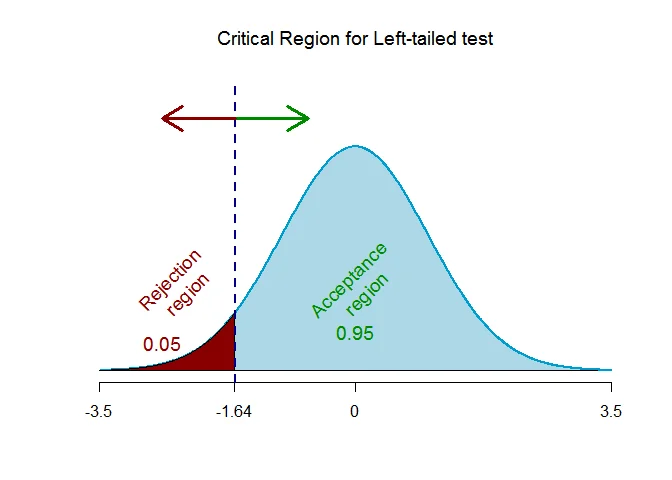
The rejection region (i.e. critical region) is $\text{Z < -1.64}$.
Step 5 Computation
The test statistic under the null hypothesis is
$$ \begin{aligned} Z_{obs}&= \frac{(\hat{p}_1-\hat{p}_2)-(p_1-p_2)}{\sqrt{\frac{\hat{p}(1-\hat{p})}{n_1}+\frac{\hat{p}(1-\hat{p})}{n_2}}}\\ &= \frac{(0.383-0.439)-0}{\sqrt{\frac{0.413*(1-0.413)}{900}+\frac{0.413*(1-0.413)}{1025}}}\\ &= -2.476 \end{aligned} $$
Step 6 Decision (Traditional approach)
The rejection region (i.e. critical region) is $\text{Z < -1.64}$. The test statistic is $Z_{obs} =-2.476$ which falls $inside$ the critical region, we $\textit{reject}$ the null hypothesis.
OR
Step 6 Decision ($p$-value approach)
The test is $\text{left-tailed}$ test, so the p-value is the area to the $\text{left}$ of the test statistic ($Z_{obs}=-2.476$) is p-value = $0.0066$.
The p-value is $0.0066$ which is $\textit{less than}$ the significance level of $\alpha = 0.05$, we $\textit{reject}$ the null hypothesis.
Interpretation
There is enough evidence to conclude that percetage of women who use smartphones is less than the percentage of men who use smartphones.
Example 2
A simple random sample of front-seat occupants involved in car crashes is obtained. Among 2823 occupants not wearing seat belts, 31 were killed. Among 7765 occupants wearing seat belts, 16 were killed. The claim is that the fatality rate is higher for those not wearing seat belts. Are Seat Belts Effective? Use $\alpha = 0.01$.
Solution
Let $p_1$ be the proportion of occupants not wearing seat belts and $p_2$ be the proportion of occupants wearing seat belts.
Given that number of front-seat occupants not wearing seat belt $n_1 = 2823$ among them $X_1= 31$ were killed and the number of front-seat occupants wearing seat belt $n_2=7765$ among them $X_2=16$ were killed.
The estimated sample proportions are $\hat{p}_1=\frac{X_1}{n_1}=\frac{31}{2823}=0.011$.
$\hat{p}_2=\frac{X_2}{n_2}=\frac{16}{7765}=0.002$.
The pooled estimate of sample proportion is $\hat{p} =\frac{X_1+X_2}{n_1+n_2}=\frac{31+16}{2823+7765} =0.004$
The claim that the fatality rate is higher for those not wearing seat belts can be expressed as $p_1 > p_2$.
Step 1 State the hypothesis testing problem
The hypothesis testing problem is
$H_0 : p_1 = p_2$ against $H_1 : p_1 > p_2$ ($\textit{right-tailed}$)
Step 2 Define test statistic
The test statistic for testing above hypothesis testing problem is
$$ \begin{aligned} Z & =\frac{(\hat{p}_1-\hat{p}_2)-(p_1-p_2)}{\sqrt{\frac{\hat{p}(1-\hat{p})}{n_1}+\frac{\hat{p}(1-\hat{p})}{n_2}}}. \end{aligned} $$
The test statistic $Z$ follows standard normal distribution $N(0,1)$.
Step 3 Specify the level of significance
The significance level is $\alpha = 0.01$.
Step 4 Determine the critical value
As the alternative hypothesis is $\textit{right-tailed}$, the critical value of $Z$ $\text{ is }$ $\text{2.33}$ (From Normal Statistical Table).
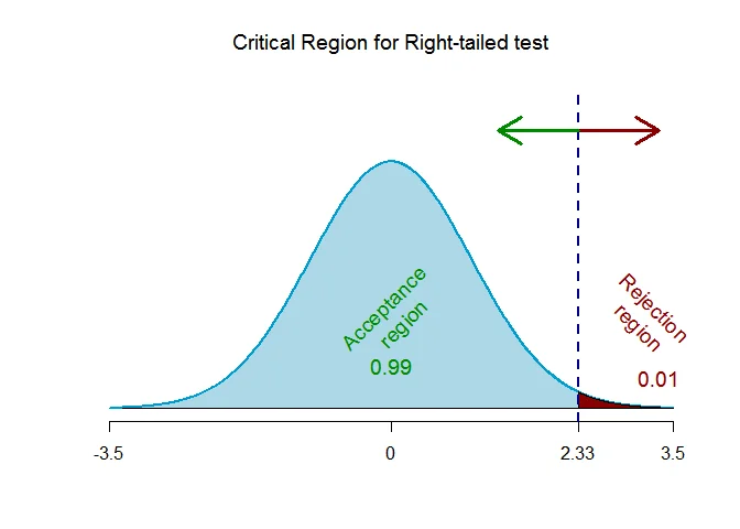
The rejection region (i.e. critical region) is $\text{Z > 2.33}$.
Step 5 Computation
The test statistic under the null hypothesis is
$$ \begin{aligned} Z_{obs}&= \frac{(\hat{p}_1-\hat{p}_2)-(p_1-p_2)}{\sqrt{\frac{\hat{p}(1-\hat{p})}{n_1}+\frac{\hat{p}(1-\hat{p})}{n_2}}}\\ &= \frac{(0.011-0.002)-0}{\sqrt{\frac{0.004*(1-0.004)}{2823}+\frac{0.004*(1-0.004)}{7765}}}\\ &= 6.106 \end{aligned} $$
Step 6 Decision (Traditional approach)
The rejection region (i.e. critical region) is $\text{Z > 2.33}$. The test statistic is $Z_{obs} =6.106$ which falls $inside$ the critical region, we $\textit{reject}$ the null hypothesis.
OR
Step 6 Decision ($p$-value approach)
The test is $\text{right-tailed}$ test, so the p-value is the area to the $\text{right}$ of the test statistic ($Z_{obs}=6.106$) is p-value = $0$.
The p-value is $0$ which is $\textit{less than}$ the significance level of $\alpha = 0.01$, we $\textit{reject}$ the null hypothesis.
Interpretation
There is enough evidence to support the claim that the fatality rate is higher for those not wearing seat belts.
Thus we conclude that the use of seat belts appears to be effective in saving lives.
Example 3
A random sample of 85 parts manufactured by machine A yields 10 defective and a random sample of 110 parts manufactured by machine B shows 15 defective.
Are the two machine differ significantly with respect to the proportion of defectives? Use $\alpha= 0.05$.
Solution
Given that $n_1 = 85$, $X_1= 10$, $n_2=110$ and $X_2=28$.
The sample proportions are $\hat{p}_1=\frac{X_1}{n_1}=\frac{10}{85}=0.118$.
$\hat{p}_2=\frac{X_2}{n_2}=\frac{28}{110}=0.255$.
The pooled estimate of sample proportion is $\hat{p} =\frac{X_1+X_2}{n_1+n_2}=\frac{10+28}{85+110} =0.195$
Step 1 State the hypothesis testing problem
The hypothesis testing problem is $H_0:$ Two machines do not differ significantly with respect to defective against $H_1:$ Two machines differ significantly with respect to proportion of defectives.
i.e., $H_0 : p_1 = p_2$ against $H_1 : p_1 \neq p_2$ ($\textit{two-tailed}$)
Step 2 Define test statistic
The test statistic for testing above hypothesis testing problem is
$$ \begin{aligned} Z & =\frac{(\hat{p}_1-\hat{p}_2)-(p_1-p_2)}{\sqrt{\frac{\hat{p}(1-\hat{p})}{n_1}+\frac{\hat{p}(1-\hat{p})}{n_2}}}. \end{aligned} $$
The test statistic $Z$ follows standard normal distribution $N(0,1)$.
Step 3 Specify the level of significance $\alpha$
The significance level is $\alpha = 0.05$.
Step 4 Determine the critical value
As the alternative hypothesis is $\textit{two-tailed}$, the critical value of $Z$ $\text{ are }$ $\text{-1.96 and 1.96}$ (From Normal Statistical Table).
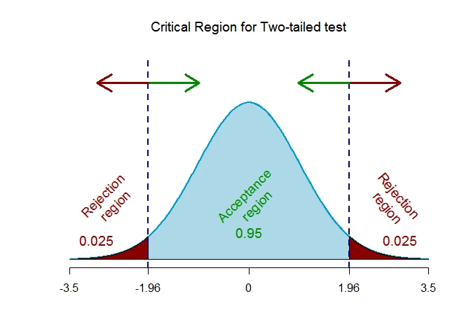
The rejection region (i.e. critical region) is $\text{Z < -1.96 or Z > 1.96}$.
Step 5 Computation
The test statistic under the null hypothesis is
$$ \begin{aligned} Z_{obs}&= \frac{(\hat{p}_1-\hat{p}_2)-(p_1-p_2)}{\sqrt{\frac{\hat{p}(1-\hat{p})}{n_1}+\frac{\hat{p}(1-\hat{p})}{n_2}}}\\ &= \frac{(0.118-0.255)-0}{\sqrt{\frac{0.195*(1-0.195)}{85}+\frac{0.195*(1-0.195)}{110}}}\\ &= -2.393 \end{aligned} $$
Step 6 Decision (Traditional approach)
The rejection region (i.e. critical region) is $\text{Z < -1.96 or Z > 1.96}$. The test statistic is $Z_{obs} =-2.393$ which falls $inside$ the critical region, we $\textit{reject}$ the null hypothesis.
OR
Decision ($p$-value approach)
The test is $\text{two-tailed}$ test, so the p-value is the area to the $\text{extreme}$ of the test statistic ($Z_{obs}=-2.393$) is p-value = $0.0167$.
The p-value is $0.0167$ which is $\textit{less than}$ the significance level of $\alpha = 0.05$, we $\textit{reject}$ the null hypothesis.
Interpretation
There is enough evidence to support the alternative hypothesis. Thus we conclude that the two machine differ significantly with respect to the proportion of defectives.