Cauchy Distribution
A continuous random variable $X$ is said to follow Cauchy
distribution with parameters $\mu$ and $\lambda$ if its probability density function is given by
$$ \begin{equation*} f(x) =\left\{ \begin{array}{ll} \frac{\lambda}{\pi}\cdot \frac{1}{\lambda^2+(x-\mu)^2}, & \hbox{$-\infty < x< \infty$;} \\ & \hbox{$-\infty < \mu< \infty$, $\lambda>0$;} \\ 0, & \hbox{Otherwise.} \end{array} \right. \end{equation*} $$
In notation it can be written as $X\sim C(\mu, \lambda)$. The parameter $\mu$ and $\lambda$ are location and scale parameters respectively.
Clearly,
$f(x)>0$ for all $x$.
Let us check whether $\int_{-\infty}^\infty f(x;\mu, \lambda); dx =1$.
$$ \begin{eqnarray*} \int_{-\infty}^\infty f(x)\; dx &=& \int_{-\infty}^\infty\frac{\lambda}{\pi}\cdot \frac{1}{\lambda^2+(x-\mu)^2} \; dx \\ &=& \frac{\lambda}{\pi}\int_{-\infty}^\infty \frac{1}{\lambda^2+(x-\mu)^2} \; dx \\ &=& \frac{\lambda}{\pi}\bigg[\frac{1}{\lambda}\tan^{-1}\bigg(\frac{x-\mu}{\lambda}\bigg)\bigg]_{-\infty}^\infty \\ &=& \frac{1}{\pi}\bigg[\tan^{-1}(\infty)-tan^{-1}(-\infty)\bigg]\\ &=& \frac{1}{\pi}\bigg[\frac{\pi}{2}-\bigg(-\frac{\pi}{2}\bigg)\bigg]\\ &=& \frac{1}{\pi}(\pi)=1. \end{eqnarray*} $$
Hence, function $f(x)$ is a legitimate probability density function.
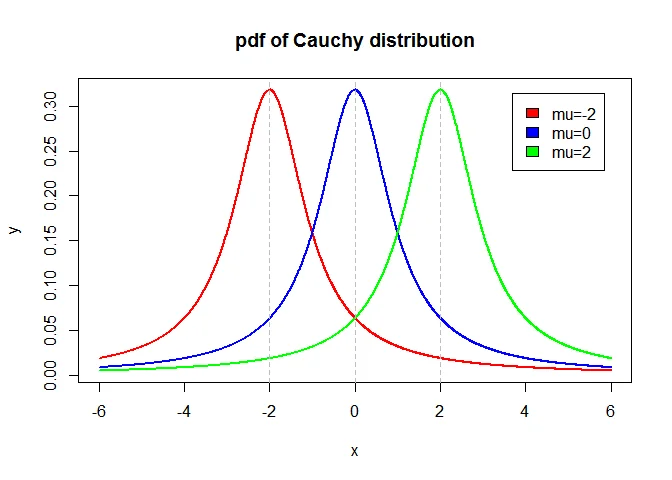
Graph of Cauchy Distribution
Graph of Cauchy distribution with various values of $\mu$ and $\lambda=1$ is as follows
Standard Cauchy Distribution
In Cauchy distribution if we take $\mu=0$ and $\lambda =1$, then the distribution is called Standard Cauchy Distribution. The p.d.f. of standard Cauchy distribution is
$$ \begin{equation*} f(x) =\left\{ \begin{array}{ll} \frac{1}{\pi}\cdot \frac{1}{1+x^2}, & \hbox{$-\infty < x< \infty$;} \\ 0, & \hbox{Otherwise.} \end{array} \right. \end{equation*} $$
Mean and variance of Cauchy Distribution
Cauchy distribution does not possesses finite moments of order greater than or equal to 1. Hence, mean and variance does not exists for Cauchy distribution.
Median of Cauchy Distribution
The median of Cauchy distribution is $\mu$.
Proof
If $M$ is the median of the distribution, then
$$ \begin{equation*} \int_{-\infty}^M f(x)\; dx =\frac{1}{2}. \end{equation*} $$
Let $\frac{x-\mu}{\lambda} = z$ $\Rightarrow$ $dx = \lambda; dz$.
$x=-\infty$ $\Rightarrow z = -\infty$ and $x = M \Rightarrow z=\frac{M-\mu}{\lambda}$. Hence, we have
$$ \begin{eqnarray*} & & \int_{-\infty}^M f(x)\; dx =\frac{1}{2} \\ &\Rightarrow& \frac{1}{\pi}\int_{-\infty}^{\frac{M-\mu}{\lambda}}\frac{dz}{1+z^2} =\frac{1}{2} \\ &\Rightarrow&\frac{1}{\pi} \bigg[\tan^{-1}z\bigg]_{-\infty}^{\frac{M-\mu}{\lambda}}=\frac{1}{2}\\ &\Rightarrow&\frac{1}{\pi} \bigg[\tan^{-1}\frac{M-\mu}{\lambda}-\tan^{-1}(-\infty)\bigg]=\frac{1}{2}\\ &\Rightarrow&\frac{1}{\pi} \bigg[\tan^{-1}\frac{M-\mu}{\lambda}-\bigg(-\frac{\pi}{2}\bigg)\bigg]=\frac{1}{2}\\ &\Rightarrow&\frac{1}{\pi} \tan^{-1}\frac{M-\mu}{\lambda}=0\\ &\Rightarrow& \frac{M-\mu}{\lambda}=0 \; \Rightarrow M =\mu. \end{eqnarray*} $$
Hence, median of the Cauchy distribution is $\mu$.
Mode of Cauchy Distribution
The mode of Cauchy distribution is $\mu$.
Proof
The probability density function of Cauchy random variable is
$$ \begin{equation}\label{eqch1} f(x; \mu, \lambda) =\left\{ \begin{array}{ll} \frac{\lambda}{\pi}\cdot \frac{1}{\lambda^2+(x-\mu)^2}, & \hbox{$-\infty < x< \infty$;} \\ & \hbox{$-\infty < \mu< \infty$, $\lambda>0$;} \\ 0, & \hbox{Otherwise.} \end{array} \right. \end{equation} $$
Mode is the value of random variable $X$ at which density function becomes maximum.
Taking $\log_e$ on both the sides of \eqref{eqch1}, we have
$$ \begin{equation}\label{eqch2} \log_e f(x) = \log (\lambda/\pi) - \log (\lambda^2+(x-\mu)^2) \end{equation} $$
By the principle of maxima and minima, differentiating \eqref{eqch2} w.r.t. $x$, and equating to zero, we get
$$ \begin{eqnarray*} \frac{\partial \log_e f(x)}{\partial x} &=& 0\; \Rightarrow \frac{-2(x-\mu)}{\lambda^2+(x-\mu)^2} =0 \\ \Rightarrow & & (x-\mu)=0\; \Rightarrow x =\mu \end{eqnarray*} $$
And
$$ \begin{eqnarray*} \frac{\partial^2 \log_e f(x)}{\partial x^2} &=& -2\bigg[\frac{[\lambda^2+(x-\mu)^2](1)-(x-\mu)[2(x-\mu)]}{[\lambda^2+(x-\mu)^2]^2}\bigg]_{x=\mu} \\ &=& -2\bigg[\frac{[\lambda^2+(x-\mu)^2](1)-2(x-\mu)^2}{[\lambda^2+(x-\mu)^2]^2}\bigg]_{x=\mu} \\ &=& -2\bigg[\frac{\lambda^2}{\lambda^4}\bigg] = \frac{-2}{\lambda^2}<0 \\ \end{eqnarray*} $$
Hence, $f(x)$ is maximum at $x=\mu$. Therefore, $ x=\mu$ is the mode of Cauchy distribution.
Quartiles of Cauchy Distribution
The Quartiles of Cauchy distributions and quartile derivation of cauchy distribution are
Proof
Let $Q_1$ be the first quartile of the distribution, then
$$ \begin{equation*} P(X\leq Q_1)=\int_{-\infty}^{Q_1} f(x)\; dx =\frac{1}{4}. \end{equation*} $$
Let $\frac{x-\mu}{\lambda} = z$ $\Rightarrow$ $dx = \lambda; dz$.\ $x=-\infty$ $\Rightarrow z = -\infty$ and $x = Q_1 \Rightarrow z=\frac{Q_1-\mu}{\lambda}$. Hence, we have
$$ \begin{eqnarray*} \int_{-\infty}^{Q_1} f(x)\; dx =\frac{1}{4} &\Rightarrow& \frac{1}{\pi}\int_{-\infty}^{\frac{Q_1-\mu}{\lambda}}\frac{dz}{1+z^2} =\frac{1}{4} \\ &\Rightarrow&\frac{1}{\pi} \bigg[\tan^{-1}z\bigg]_{-\infty}^{\frac{Q_1-\mu}{\lambda}}=\frac{1}{4}\\ &\Rightarrow&\frac{1}{\pi} \bigg[\tan^{-1}\frac{Q_1-\mu}{\lambda}-\tan^{-1}(-\infty)\bigg]=\frac{1}{4}\\ &\Rightarrow&\frac{1}{\pi} \bigg[\tan^{-1}\frac{Q_1-\mu}{\lambda}-\bigg(-\frac{\pi}{2}\bigg)\bigg]=\frac{1}{4} \end{eqnarray*} $$
$$ \begin{eqnarray*} &\Rightarrow& \tan^{-1}\frac{Q_1-\mu}{\lambda}=-\frac{\pi}{4}\\ &\Rightarrow& \frac{Q_1-\mu}{\lambda}=\tan\bigg(-\frac{\pi}{4}\bigg)=-1 \; \Rightarrow Q_1 =\mu-\lambda. \end{eqnarray*} $$
Therefore for the Cauchy distribution, first quartile $Q_1=\mu-\lambda$.
Third Quartile
Let $Q_3$ be the second quartile of the distribution, then
$$ \begin{equation*} P(X\leq Q_3)=\int_{-\infty}^{Q_3} f(x)\; dx =\frac{3}{4}. \end{equation*} $$
Let $\frac{x-\mu}{\lambda} = z$ $\Rightarrow$ $dx = \lambda; dz$.\
$x=-\infty$ $\Rightarrow z = -\infty$ and $x = Q_3 \Rightarrow z=\frac{Q_3-\mu}{\lambda}$. Hence, we have
$$ \begin{eqnarray*} \int_{-\infty}^{Q_3} f(x)\; dx =\frac{3}{4} &\Rightarrow& \frac{1}{\pi}\int_{-\infty}^{\frac{Q_3-\mu}{\lambda}}\frac{dz}{1+z^2} =\frac{3}{4} \\ &\Rightarrow&\frac{1}{\pi} \bigg[\tan^{-1}z\bigg]_{-\infty}^{\frac{Q_3-\mu}{\lambda}}=\frac{3}{4}\\ &\Rightarrow&\frac{1}{\pi} \bigg[\tan^{-1}\frac{Q_3-\mu}{\lambda}-\tan^{-1}(-\infty)\bigg]=\frac{3}{4}\\ &\Rightarrow&\frac{1}{\pi} \bigg[\tan^{-1}\frac{Q_3-\mu}{\lambda}-\bigg(-\frac{\pi}{2}\bigg)\bigg]=\frac{3}{4} \end{eqnarray*} $$
$$ \begin{eqnarray*} &\Rightarrow& \tan^{-1}\frac{Q_3-\mu}{\lambda}=\frac{\pi}{4}\\ &\Rightarrow& \frac{Q_3-\mu}{\lambda}=\tan\bigg(\frac{\pi}{4}\bigg)=1 \; \Rightarrow Q_3 =\mu+\lambda. \end{eqnarray*} $$
Therefore for the Cauchy distribution, third quartile $Q_3=\mu+\lambda$.
Hence the Quartile Deviation of Cauchy distribution is
$$ \begin{equation*} QD = \frac{Q_3-Q_1}{2} =\frac{\mu+\lambda-(\mu-\lambda)}{2}=\lambda. \end{equation*} $$
Distribution Function of Cauchy Distribution
The distribution function of Cauchy random variable is
$$ \begin{equation*} F(x) =\frac{1}{\pi}\tan^{-1}\bigg(\frac{x-\mu}{\lambda}\bigg) + \frac{1}{2}. \end{equation*} $$
Proof
$$ \begin{equation*} F(x)=P(X\leq x) = \int_{-\infty}^x f(x)\; dx. \end{equation*} $$
Let $\frac{x-\mu}{\lambda} = z$ $\Rightarrow$ $dx = \lambda; dz$.\
$x=-\infty$ $\Rightarrow z = -\infty$ and $x = x \Rightarrow z=\frac{x-\mu}{\lambda}$. Hence, we have
$$ \begin{eqnarray*} % \nonumber to remove numbering (before each equation) F(x) & = & \frac{1}{\pi}\int_{-\infty}^{\frac{x-\mu}{\lambda}}\frac{dz}{1+z^2}\\ & = &\frac{1}{\pi} \bigg[\tan^{-1}z\bigg]_{-\infty}^{\frac{x-\mu}{\lambda}}\\ & = &\frac{1}{\pi} \bigg[\tan^{-1}\bigg(\frac{x-\mu}{\lambda}\bigg)-\tan^{-1}(-\infty)\bigg]\\ & = &\frac{1}{\pi} \bigg[\tan^{-1}\bigg(\frac{x-\mu}{\lambda}\bigg)-\bigg(-\frac{\pi}{2}\bigg)\bigg]\\ & = & \frac{1}{\pi}\tan^{-1}\bigg(\frac{x-\mu}{\lambda}\bigg) + \frac{1}{2}. \end{eqnarray*} $$
The distribution function of Cauchy distribution is
$$ \begin{equation*} F(x) =\frac{1}{\pi}\tan^{-1}\bigg(\frac{x-\mu}{\lambda}\bigg) + \frac{1}{2}. \end{equation*} $$
MGF of Cauchy Distribution
Moment generating function of Cauchy distribution does not exists
Characteristics Function of Cauchy Distribution
The characteristics function of cauchy distribution is
$$ \phi_X(t)= e^{i\mu t -\lambda|t|}. $$
Proof
If $Y$ is standard Cauchy variate then its characteristics function is
$$ \begin{equation}\label{cfc1} \phi_Y(t) = \int_{-\infty}^\infty e^{ity} f(y)\; dx=\frac{1}{\pi}\int_{-\infty}^\infty \frac{e^{ity}}{1+y^2}\; dy. \end{equation} $$
Consider the p.d.f. of standard Laplace distribution
$$ \begin{equation*} f_1(z) = \frac{1}{2} e^{-|z|}, \; \; -\infty < z< \infty. \end{equation*} $$
The characteristics function of $Z$ is
$$ \begin{equation*} \phi_1(t) = E(e^{itz}) = \frac{1}{1+t^2}. \end{equation*} $$
Here, $\phi_1(t)$ is absolutely integrable in $(-\infty, \infty)$, we have by Inversion Theorem,
$$ \begin{eqnarray*} f_1(z) &=& \frac{1}{2\pi} \int_{-\infty}^\infty e^{-itz} \phi_1(t)\;dt \\ &=& \frac{1}{2\pi} \int_{-\infty}^\infty \frac{e^{-itz}}{1+t^2}\; dt\\ \therefore \frac{1}{2}e^{-|z|} & = &\frac{1}{2\pi} \int_{-\infty}^\infty \frac{e^{-itz}}{1+t^2}\; dt\\ e^{-|z|} & = &\frac{1}{\pi} \int_{-\infty}^\infty \frac{e^{itz}}{1+t^2}\; dt\qquad \text{ changing $t$ to $-t$} \end{eqnarray*} $$
Interchanging $t$ and $z$, we get
$$ \begin{equation}\label{cfc2} e^{-|t|} = \frac{1}{\pi} \int_{-\infty}^\infty \frac{e^{itz}}{1+z^2}\; dz \end{equation} $$
From \eqref{cfc1} and \eqref{cfc2}, we get
$$ \begin{equation*} \phi_Y(t) = e^{-|t|}. \end{equation*} $$
Let $X\sim C(\mu, \lambda)$, then $Y=\frac{X-\mu}{\lambda}\sim C(0,1)$. Hence, $X=\mu + \lambda Y$ has a characteristics function
$$ \begin{eqnarray*} \phi_X(t)& = & E(e^{itX})\\ & = &E(e^{it(\mu+\lambda Y)})\\ & = & e^{i\mu t}E(e^{it\lambda Y}) \\ & = & e^{i\mu t}\phi_Y(t\lambda)\\ & =& e^{i\mu t}e^{-\lambda|t|}\\ & =& e^{i\mu t -\lambda|t|}. \end{eqnarray*} $$
Additive Property of Cauchy Distribution
If $X_1$ and $X_2$ are two independent Cauchy random variables with parameters $(\mu_1, \lambda_1)$ and $(\mu_2, \lambda_2)$ respectively, then $X_1+X_2$ is a Cauchy random variable with parameter $(\mu_1+\mu_2, \lambda_1+\lambda_2)$.
Proof
The characteristics function of $X_1$ and $X_2$ are $\phi_{X_1}(t) =e^{i\mu_1 t -\lambda_1|t|}$ and $\phi_{X_1}(t) = e^{i\mu_2 t-\lambda_2|t|}$ respectively.
Hence the characteristics function of $X_1+X_2$ is
$$ \begin{eqnarray*} \phi_{X_1+X_2} (t) &=& \phi_{X_1}(t)\cdot \phi_{X_2}(t), \quad \text{ $X_1$ and $X_2$ are independent} \\ &=& e^{i\mu_1 t -\lambda_1|t|}\cdot e^{i\mu_2 t-\lambda_2|t|}\\ & = & e^{i(\mu_1+\mu_2) t -(\lambda_1+\lambda_2)|t|}. \end{eqnarray*} $$
Hence by uniqueness theorem of characteristics function, $X_1+X_2$ follows Cauchy distribution with parameters $\mu_1+\mu_2$ and $\lambda_1+\lambda_2$.
Result
Let $X_1, X_2, \cdots, X_n$ be a sample of $n$ independent observations from Cauchy distribution such that $X_j \sim C(\lambda_j, \mu_j)$, $j=1,2\cdots, n$. Then $\overline{X}$, sample mean follows a Cauchy distribution with parameters $\overline{\lambda}$ and $\overline{\mu}$, where $\overline{\lambda}= \frac{1}{n}\sum_{j=1}^n \lambda_j$ and $\overline{\mu} =\frac{1}{n}\sum_{j=1}^n \mu_j$.
Reciprocal of standard Cauchy distribution
Let $X$ be a random variable having Cauchy distribution with parameter $\mu=0$ and $\lambda=1$. Find the distribution of $\frac{1}{X}$. Identify the distribution.
Proof
$X\sim C(0, 1)$. Therefore, the p.d.f. of $X$ is $f(x)=\frac{1}{\pi}\cdot \frac{1}{1+x^2}$, $-\infty < x< \infty$. Let $y=\frac{1}{x}$. Therefore $dx = -\frac{1}{y^2}dy$. Hence, p.d.f. of $Y$ is
$$ \begin{eqnarray*} f(y) &=& f(x)\cdot\bigg|\frac{dx}{dy} \bigg|\\ &=& \frac{1}{\pi}\cdot \frac{1}{1+(1/y^2)}\cdot \frac{1}{y^2}\\ &=& \frac{1}{\pi}\cdot \frac{1}{1+y^2},\quad -\infty < y < \infty, \end{eqnarray*} $$
which is the p.d.f. of standard Cauchy distribution. Hence $Y\sim C(0,1)$ distribution.
Result
A random variable $X$ has a standard Cauchy distribution. Find the p.d.f. of $X^2$ and identify the distribution.
Solution
Let $X\sim C(0,1)$. The p.d.f. of $X$ is $f(x) =\frac{1}{\pi}\cdot\frac{1}{1+x^2}$, $-\infty < x< \infty$. Let $Y=X^2$.
Distribution function of $Y$ is given by
$$ \begin{eqnarray*} G(y) &=& P(Y\leq y) \\ &=& P(X^2\leq y)\\ &=& P(-\sqrt(y)\leq X\leq \sqrt{y})\\ &=& \int_{-\sqrt{y}}^{\sqrt{y}}f(x) \; dx\\ &=& \frac{1}{\pi}\int_{-\sqrt{y}}^{\sqrt{y}}\frac{1}{1+x^2} \; dx\\ &=& \frac{2}{\pi}\int_{0}^{\sqrt{y}}\frac{1}{1+x^2} \; dx\\ &=& \frac{2}{\pi}\big[\tan^{-1}x\big]_{0}^{\sqrt{y}}\\ &=& \frac{2}{\pi}\cdot\tan^{-1}\sqrt{y}. \end{eqnarray*} $$
Hence, p.d.f. of $Y$ is
$$ \begin{eqnarray*} g(y) &=& \frac{d}{dy} G(y) \\ &=& \frac{2}{\pi}\cdot\frac{1}{1+(\sqrt{y})^2}\cdot \frac{1}{2\sqrt{y}}\\ &=& \frac{2}{\pi}\cdot\frac{y^{-1/2}}{1+y}\\ &=& \frac{1}{\pi}\cdot\frac{y^{\frac{1}{2}-1}}{(1+y)^{\frac{1}{2}+\frac{1}{2}}}\\ &=& \frac{1}{B\big(\frac{1}{2},\frac{1}{2}\big)}\cdot\frac{y^{\frac{1}{2}-1}}{(1+y)^{\frac{1}{2}+\frac{1}{2}}} \end{eqnarray*} $$
which is the p.d.f. of $\beta$ distribution of second kind with $m=\frac{1}{2},n=\frac{1}{2}$, i.e., $F$ distribution with (1,1) degrees of freedom. Hence, $Y=X^2 \sim \beta_2\big(\frac{1}{2},\frac{1}{2}\big)= F(1,1)$.
Ratio of independent standard normal
Let $X\sim N(0,1)$ and $Y\sim N(0,1)$ be independent random variable. Find the distribution of $X/Y$.
Proof
Let $X\sim N(0,1)$ and $Y\sim N(0,1)$. Moreover, $X$ and $Y$ are independently distributed. Therefore, the joint p.d.f. of $X$ and $Y$ is given by
$$ \begin{eqnarray*} f(x,y) &=& f(x)\cdot f(y) \\ &=& \frac{1}{2\pi} e^{-\frac{1}{2}(x^2+y^2)}. \end{eqnarray*} $$
Let $U=X/Y$ and $V=Y$. Hence $X=UV$ and $Y=V$. Hence, the Jacobian of the transformation is
$$ \begin{equation*} J=\bigg|\frac{\partial(x,y)}{\partial(u,v)}\bigg|=\bigg| \begin{array}{cc} v & u \\ 0 & 1 \\ \end{array} \bigg|=|v|. \end{equation*} $$
Hence the joint p.d.f. of $U$ and $V$ is
$$ \begin{eqnarray*} f(u,v) &=& f(x,y)\cdot |J| \\ &=& \frac{1}{2\pi} e^{-\frac{1}{2}(u^2v^2+v^2)}|v|. \end{eqnarray*} $$
Hence, the marginal p.d.f. of $U$ is
$$ \begin{eqnarray*} f(u) &=& \int_{-\infty}^\infty f(u,v) \; dv \\ &=& \frac{1}{2\pi} \int_{-\infty}^\infty e^{-\frac{1}{2}(u^2+1)v^2}|v|\; dv\\ &=& \frac{1}{\pi} \int_{0}^\infty e^{-\frac{1}{2}(u^2+1)v^2}v\; dv\\ & & \qquad \qquad \int_{0}^\infty e^{-ax^2}x^{2n-1}\; dx=\frac{\Gamma(n)}{2a^n}\\ &=& \frac{1}{\pi} \frac{\Gamma(2)}{(2(1+u^2)/2)^{2/2}}\\ &=& \frac{1}{\pi} \frac{1}{1+u^2}. \end{eqnarray*} $$
which is the p.d.f. of Cauchy distribution with parameter $\mu=0$ and $\lambda =1$. Hence $X/Y \sim C(0,1)$ distribution.
Example
Let $X\sim C(\mu, \lambda)$. Let $X_1$ and $X_2$ are two independent observations on $X$. Find
- $P[X_1+X_2> 2(\mu+\lambda)]$
- $P[X_1+X_2< 2(\mu-\lambda)]$
- $P[2(\mu-\lambda) < X_1+X_2< 2(\mu+\lambda)]$.
Solution
Let $X_1\sim C(\mu,\lambda)$ and $X_2\sim C(\mu, \lambda)$. Moreover $X_1$ and $X_2$ are independent. Hence $\frac{X_1+X_2}{2}=\overline{X} \sim C(\mu, \lambda)$. Hence
$$ \begin{eqnarray*} P[X_1+X_2> 2(\mu+\lambda)] &=& P[\overline{X}> (\mu+\lambda)] \\ &=& P[\overline{X}> Q_3],\quad \text{ since $Q_3=\mu+\lambda$} \\ &=& 1-P[\overline{X}\leq Q_3]\\ &=& 1-\frac{3}{4}=\frac{1}{4}. \end{eqnarray*} $$
Conclusion
Hope you like above detailed article on Cauchy distribution with proof for standard cauchy distibution,addictive property of cauchy distribution and many more.