Introduction to Exponential Distribution
The exponential distribution is a continuous probability distribution used to model the time between events in a Poisson process. It is widely used in reliability engineering, queuing theory, survival analysis, and modeling waiting times. The exponential distribution is the only continuous distribution with the memoryless property, making it unique among continuous distributions.
Definition of Exponential Distribution
A continuous random variable $X$ is said to have an exponential distribution with parameter $\theta$ if its probability density function (PDF) is given by:
$$ \begin{equation*} f(x)=\left{ \begin{array}{ll} \theta e^{-\theta x}, & \hbox{$x\geq 0;\theta>0$;} \ 0, & \hbox{Otherwise.} \end{array} \right. \end{equation*} $$
where $\theta > 0$ is the rate parameter.
Notation: $X\sim \exp(\theta)$
Alternative Form
Another common form of the exponential distribution uses the parameter $\lambda = 1/\theta$ (scale parameter):
$$ \begin{equation*} f(x)=\left{ \begin{array}{ll} \frac{1}{\lambda} e^{-\frac{x}{\lambda}}, & \hbox{$x\geq 0;\lambda>0$;} \ 0, & \hbox{Otherwise.} \end{array} \right. \end{equation*} $$
Notation: $X\sim \exp(\lambda)$
Standard Exponential Distribution
When $\theta = 1$ (or $\lambda = 1$), we have the standard exponential distribution:
$$ \begin{equation*} f(x)=\left{ \begin{array}{ll} e^{-x}, & \hbox{$x\geq 0$;} \ 0, & \hbox{Otherwise.} \end{array} \right. \end{equation*} $$
Probability Density Function (PDF)
The PDF of the exponential distribution is:
$$f(x) = \theta e^{-\theta x}, \quad x \geq 0$$
Graph of PDF of Exponential Distribution
Following is the graph of the probability density function of exponential distribution with parameter $\theta=0.4$:
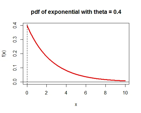
The PDF shows a decreasing curve that starts at $\theta$ (when $x=0$) and approaches zero as $x$ increases. The shape is determined by the rate parameter $\theta$.
Cumulative Distribution Function (CDF)
The cumulative distribution function (CDF) gives the probability that $X$ is less than or equal to $x$:
$$ \begin{equation*} F(x)=\left{ \begin{array}{ll} 1- e^{-\theta x}, & \hbox{$x\geq 0;\theta>0$;} \ 0, & \hbox{$x < 0$.} \end{array} \right. \end{equation*} $$
Proof
$$ \begin{eqnarray*} F(x) &=& P(X\leq x) \ &=& \int_0^x f(t);dt\ &=& \theta \int_0^x e^{-\theta t};dt\ &=& \theta \bigg[-\frac{e^{-\theta t}}{\theta}\bigg]_0^x \ &=& 1-e^{-\theta x} \end{eqnarray*} $$
Graph of CDF of Exponential Distribution
Following is the graph of the cumulative density function of exponential distribution with parameter $\theta=0.4$:
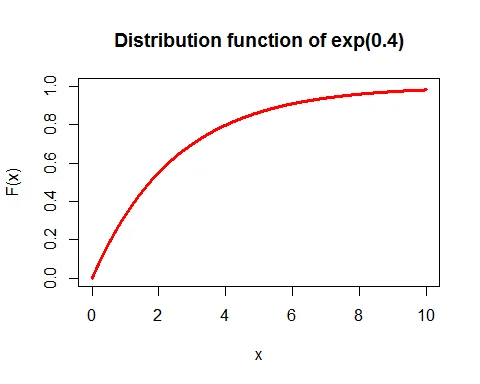
The CDF shows an increasing function starting at 0 and approaching 1 as $x$ increases.
Key Properties of Exponential Distribution
Mean of Exponential Distribution
The mean of an exponential random variable is:
$$E(X) = \frac{1}{\theta}$$
Proof
$$ \begin{eqnarray*} E(X) &=& \int_0^\infty x\theta e^{-\theta x}; dx\ &=& \theta \int_0^\infty x^{2-1}e^{-\theta x}; dx\ &=& \theta \frac{\Gamma(2)}{\theta^2}\quad (\text{Using }\int_0^\infty x^{n-1}e^{-\theta x}; dx = \frac{\Gamma(n)}{\theta^n} )\ &=& \frac{1}{\theta} \end{eqnarray*} $$
Variance of Exponential Distribution
The variance of an exponential random variable is:
$$V(X) = \frac{1}{\theta^2}$$
Proof
First, find $E(X^2)$:
$$ \begin{eqnarray*} E(X^2) &=& \int_0^\infty x^2\theta e^{-\theta x}; dx\ &=& \theta \int_0^\infty x^{3-1}e^{-\theta x}; dx\ &=& \theta \frac{\Gamma(3)}{\theta^3}\ &=& \frac{2}{\theta^2} \end{eqnarray*} $$
Then:
$$ \begin{eqnarray*} V(X) &=& E(X^2) -[E(X)]^2\ &=&\frac{2}{\theta^2}-\bigg(\frac{1}{\theta}\bigg)^2\ &=&\frac{1}{\theta^2} \end{eqnarray*} $$
Standard Deviation
$$\sigma = \sqrt{V(X)} = \frac{1}{\theta}$$
Note that for exponential distribution: Mean = Standard Deviation = $\frac{1}{\theta}$
Raw Moments
The $r^{th}$ raw moment of an exponential random variable is:
$$\mu_r^\prime = \frac{r!}{\theta^r}$$
This gives us:
- $\mu_1^\prime = E(X) = \frac{1}{\theta}$
- $\mu_2^\prime = E(X^2) = \frac{2}{\theta^2}$
- $\mu_3^\prime = E(X^3) = \frac{6}{\theta^3}$
Moment Generating Function (MGF)
The moment generating function of an exponential random variable is:
$$M_X(t) = \bigg(1- \frac{t}{\theta}\bigg)^{-1}, \quad \text{for } t < \theta$$
Proof
$$ \begin{eqnarray*} M_X(t) &=& E(e^{tX}) \ &=& \int_0^\infty e^{tx}\theta e^{-\theta x}; dx\ &=& \theta \int_0^\infty e^{-(\theta-t) x}; dx\ &=& \theta \bigg[-\frac{e^{-(\theta-t) x}}{\theta-t}\bigg]_0^\infty\ &=& \frac{\theta }{\theta-t}, \quad \text{for } t<\theta\ &=& \bigg(1- \frac{t}{\theta}\bigg)^{-1} \end{eqnarray*} $$
Characteristic Function
The characteristic function of an exponential random variable is:
$$\phi_X(t) = \bigg(1- \frac{it}{\theta}\bigg)^{-1}, \quad \text{for } t < \theta$$
The Memoryless Property
The memoryless property (or lack of memory) is a unique and defining characteristic of the exponential distribution among continuous distributions.
Definition
For any $s \geq 0$ and $t \geq 0$:
$$P(X>s+t|X>t) = P(X>s)$$
This means the probability that we must wait an additional time $s$ beyond time $t$ (given that we’ve already waited time $t$) is the same as the probability of waiting time $s$ from the start.
Proof
$$ \begin{eqnarray*} P(X>s+t|X>t) &=& \frac{P(X>s+t,X>t)}{P(X>t)}\ &=&\frac{P(X>s+t)}{P(X>t)}\ &=& \frac{1-F(s+t)}{1-F(t)}\ &=& \frac{e^{-\theta (s+t)}}{e^{-\theta t}}\ &=& e^{-\theta s}\ &=& P(X>s) \end{eqnarray*} $$
Practical Interpretation
If the time until an event (like a lightbulb failing) follows an exponential distribution, then knowing how long the system has already been operating provides no information about how much longer it will continue to operate. The “future” is independent of the “past.”
This is in contrast to aging systems where the probability of failure increases with age.
Relationship to Poisson Process
The exponential distribution describes the time between consecutive events in a Poisson process with rate $\lambda$. If events occur according to a Poisson process, then the waiting times between events are exponentially distributed with parameter $\theta = \lambda$.
Properties Summary Table
| Property | Formula |
|---|---|
| $f(x) = \theta e^{-\theta x}$ | |
| CDF | $F(x) = 1 - e^{-\theta x}$ |
| Support | $[0, \infty)$ |
| Mean | $E(X) = \frac{1}{\theta}$ |
| Median | $\frac{\ln 2}{\theta}$ |
| Mode | $0$ |
| Variance | $V(X) = \frac{1}{\theta^2}$ |
| Std. Deviation | $\sigma = \frac{1}{\theta}$ |
| Coefficient of Variation | $1$ |
| Skewness | $2$ |
| Kurtosis | $9$ |
| MGF | $M_X(t) = (1 - t/\theta)^{-1}$ |
| CF | $\phi_X(t) = (1 - it/\theta)^{-1}$ |
Examples with Solutions
Example 1: Machine Repair Time
Problem: The time (in hours) required to repair a machine is exponentially distributed with parameter $\lambda = 1/2$. Find:
a. The probability that a repair time exceeds 4 hours b. The probability that a repair time takes at most 3 hours c. The probability that a repair time takes between 2 to 4 hours d. The conditional probability that a repair takes at least 10 hours, given that its duration exceeds 9 hours
Solution:
Let $X$ denote the time (in hours) required to repair a machine. Given: $X$ is exponentially distributed with $\lambda = 1/2$, so $\theta = 2$.
The PDF is: $f(x) = 2e^{-2x}$, $x > 0$
The CDF is: $F(x) = 1 - e^{-2x}$
Part (a): $P(X > 4)$
$$P(X > 4) = 1 - F(4) = 1 - (1 - e^{-2 \times 4}) = e^{-8} \approx 0.0003$$
The probability that repair exceeds 4 hours is approximately 0.03%.
Part (b): $P(X \leq 3)$
$$P(X \leq 3) = F(3) = 1 - e^{-2 \times 3} = 1 - e^{-6} \approx 0.9975$$
The probability that repair takes at most 3 hours is approximately 99.75%.
Part (c): $P(2 < X < 4)$
$$P(2 < X < 4) = F(4) - F(2)$$ $$= (1 - e^{-8}) - (1 - e^{-4})$$ $$= e^{-4} - e^{-8}$$ $$\approx 0.0183 - 0.0003 = 0.018$$
The probability that repair takes between 2 to 4 hours is approximately 1.8%.
Part (d): $P(X \geq 10 | X > 9)$ using Memoryless Property
Using the memoryless property: $$P(X \geq 10 | X > 9) = P(X > 9 + 1 | X > 9) = P(X > 1)$$ $$= 1 - F(1) = e^{-2 \times 1} = e^{-2} \approx 0.1353$$
The probability is approximately 13.53%.
Example 2: Machine Failure Time
Problem: The time to failure $X$ of a machine has exponential distribution with PDF:
$$f(x) = 0.01e^{-0.01x}, \quad x > 0$$
Find: a. The distribution function of $X$ b. The probability that the machine fails between 100 and 200 hours c. The probability that the machine fails before 100 hours d. The value of $x$ such that $P(X > x) = 0.5$ (median)
Solution:
Let $X$ denote the time to failure of a machine. Given: $\lambda = 0.01$, so $\theta = 0.01$.
Part (a): Distribution Function
$$F(x) = 1 - e^{-0.01x}$$
Part (b): $P(100 < X < 200)$
$$P(100 < X < 200) = F(200) - F(100)$$ $$= (1 - e^{-2}) - (1 - e^{-1})$$ $$= e^{-1} - e^{-2}$$ $$\approx 0.3679 - 0.1353 = 0.2326$$
The probability that the machine fails between 100 and 200 hours is approximately 23.26%.
Part (c): $P(X \leq 100)$
$$P(X \leq 100) = F(100) = 1 - e^{-0.01 \times 100} = 1 - e^{-1} \approx 0.6321$$
The probability that the machine fails before 100 hours is approximately 63.21%.
Part (d): Median (where $P(X > x) = 0.5$)
$$P(X > x) = 0.5$$ $$1 - F(x) = 0.5$$ $$e^{-0.01x} = 0.5$$ $$-0.01x = \ln(0.5)$$ $$x = -\frac{\ln(0.5)}{0.01} = \frac{0.693}{0.01} \approx 69.3 \text{ hours}$$
The median lifetime is approximately 69.3 hours.
Example 3: Lightbulb Lifetime and Memoryless Property
Problem: The lifetime of a lightbulb (in hours) has an exponential distribution with rate parameter $\theta = 1/100$ hours. The lightbulb has been on for 50 hours. Find the probability that the bulb survives at least another 100 hours.
Solution:
Let $X$ denote the lifetime of a lightbulb. Given: $X \sim \exp(1/100)$
Using the memoryless property:
$$P(X > 150 | X > 50) = P(X > 100 + 50 | X > 50) = P(X > 100)$$ $$= 1 - F(100) = 1 - (1 - e^{-100/100})$$ $$= e^{-1} \approx 0.3679$$
The probability that the bulb survives another 100 hours is approximately 36.79%.
This result is independent of the fact that it has already been on for 50 hours;the distribution “forgets” the past!
Sum of Exponential Variates
If $X_i, i=1,2,\cdots, n$ are independent identically distributed exponential random variables with parameter $\theta$, then:
$$\sum_{i=1}^n X_i \sim \text{Gamma}(\alpha = n, \beta = 1/\theta)$$
Proof
The MGF of each $X_i$ is: $M_{X_i}(t) = (1 - t/\theta)^{-1}$
The MGF of the sum is:
$$M_Z(t) = \prod_{i=1}^n M_{X_i}(t) = [(1 - t/\theta)^{-1}]^n = (1 - t/\theta)^{-n}$$
This is the MGF of a Gamma distribution with shape parameter $\alpha = n$ and rate parameter $\theta$.
When to Use Exponential Distribution
The exponential distribution is appropriate when:
- Waiting Times: Time until next event (customer arrival, equipment failure)
- Lifetime Analysis: Reliability of equipment with constant failure rate
- Queuing Systems: Service times in queue or waiting times
- Radioactive Decay: Time until radioactive particle decays
- Poisson Processes: Time between events in a Poisson process
- No Aging Effect: System has no memory of past operation
- Manufacturing: Time to failure for non-repairable items
Applications
- Reliability Engineering: Equipment failure rates and MTBF (Mean Time Between Failures)
- Queuing Theory: Customer service times and arrival processes
- Insurance: Claims processing times
- Telecommunications: Call duration and inter-arrival times
- Network Traffic: Packet arrival times
- Survival Analysis: Time to event in medical studies
- Inventory Management: Time until stock depletion
Related Distributions
Related Continuous Distributions:
- Gamma Distribution - Generalization of exponential
- Weibull Distribution - For reliability analysis
- Normal Distribution - Symmetric alternative
- Poisson Distribution - Discrete analog
Related Concepts:
- Expected Value and Variance - Key statistical measures
- Continuous Distributions Guide - Continuous distribution hub
- Probability Distributions Complete Guide - Full reference
Connection to Other Distributions
- Gamma Distribution: Sum of exponential variates
- Poisson Distribution: If events follow Poisson process, time between events is exponential
- Weibull Distribution: Exponential is special case ($k=1$)
- Chi-square Distribution: Related through Gamma distribution
References
-
Montgomery, D.C., & Runger, G.C. (2018). Applied Statistics for Engineers and Scientists (6th ed.). John Wiley & Sons. - Exponential distribution in reliability analysis, system lifetimes, and failure time modeling.
-
Anderson, D.R., Sweeney, D.J., & Williams, T.A. (2018). Statistics for Business and Economics (14th ed.). Cengage Learning. - Exponential distribution applications in modeling waiting times and service processes.
Conclusion
The exponential distribution is fundamental to probability and statistics, especially in reliability analysis, queuing theory, and survival analysis. Its unique memoryless property distinguishes it from all other continuous distributions and makes it the natural choice for modeling time-to-event data in systems with constant failure rates. Understanding its properties, the MGF, and practical applications is essential for engineers and statisticians working with reliability and queuing problems.
The simplicity of the exponential distribution;just one parameter;combined with its powerful theoretical properties makes it a cornerstone of probabilistic modeling in practical applications.