Introduction to Gamma Distribution
The gamma distribution is a versatile continuous probability distribution used to model a wide variety of positive-valued random variables. It is particularly useful for modeling time-to-event data, waiting times, and continuous random variables with positive support. The gamma distribution is widely used in reliability engineering, insurance, telecommunications, and scientific research due to its flexibility.
Definition of Gamma Distribution
A continuous random variable $X$ is said to have a gamma distribution with parameters $\alpha$ (shape) and $\beta$ (scale) if its probability density function (PDF) is given by:
$$ \begin{align*} f(x) &= \begin{cases} \frac{1}{\beta^\alpha\Gamma(\alpha)}x^{\alpha -1}e^{-x/\beta}, & x > 0;\alpha, \beta > 0; \ 0, & \text{Otherwise} \end{cases} \end{align*} $$
where $\Gamma(\alpha)=\int_0^\infty x^{\alpha-1}e^{-x}; dx$ is the gamma function.
Notation: $X\sim G(\alpha, \beta)$ or $X\sim \text{Gamma}(\alpha, \beta)$
Parameters
- $\alpha$ (Shape Parameter): Controls the shape of the distribution (must be $\alpha > 0$)
- $\beta$ (Scale Parameter): Controls the scale/spread of the distribution (must be $\beta > 0$)
Gamma Function
The gamma function is defined as:
$$\Gamma(\alpha) = \int_0^\infty x^{\alpha-1}e^{-x}; dx$$
Properties of Gamma Function
- $\Gamma(1) = 1$
- $\Gamma(n) = (n-1)!$ for positive integers $n$
- $\Gamma(\alpha + 1) = \alpha \Gamma(\alpha)$
- $\Gamma(1/2) = \sqrt{\pi}$
- $\Gamma(3/2) = \frac{1}{2}\Gamma(1/2) = \frac{\sqrt{\pi}}{2}$
Alternative Forms of Gamma Distribution
Form 1: With Rate Parameter
Another common form uses $\alpha$ (shape) and $\lambda = 1/\beta$ (rate parameter):
$$ f(x)=\left{ \begin{array}{ll} \frac{\lambda^\alpha}{\Gamma(\alpha)}x^{\alpha -1}e^{-\lambda x}, & \hbox{$x>0;\alpha, \lambda >0$;} \ 0, & \hbox{Otherwise.} \end{array} \right. $$
One-Parameter Gamma Distribution
Letting $\beta = 1$ gives the one-parameter gamma distribution:
$$ f(x)=\left{ \begin{array}{ll} \frac{1}{\Gamma(\alpha)}x^{\alpha -1}e^{-x}, & \hbox{$x>0;\alpha >0$;} \ 0, & \hbox{Otherwise.} \end{array} \right. $$
Graph of Gamma Distribution
Following is the graph of probability density function (PDF) of gamma distribution with parameter $\alpha=1$ and $\beta=1,2,4$:
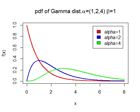
The graph shows how the distribution’s shape changes with different scale parameters while keeping the shape parameter constant.
Probability Density Function (PDF)
The PDF of the gamma distribution is:
$$f(x) = \frac{1}{\beta^\alpha\Gamma(\alpha)}x^{\alpha -1}e^{-x/\beta}, \quad x > 0$$
Properties of the PDF
- Support: All positive real numbers $(0, \infty)$
- Shape: Determined by the shape parameter $\alpha$
- When $\alpha < 1$: Decreasing curve (like exponential)
- When $\alpha = 1$: Exponential distribution
- When $\alpha > 1$: Unimodal with mode at $(\alpha-1)\beta$
- Scale: Determined by parameter $\beta$
- Larger $\beta$ stretches the distribution
- Smaller $\beta$ compresses the distribution
Cumulative Distribution Function (CDF)
The cumulative distribution function (CDF) is:
$$F(x) = P(X \leq x) = \int_0^x f(t); dt$$
For the gamma distribution, the CDF does not have a closed-form solution in terms of elementary functions. It is typically expressed in terms of the lower incomplete gamma function or evaluated numerically.
Key Properties of Gamma Distribution
Mean of Gamma Distribution
The mean of $G(\alpha,\beta)$ distribution is:
$$E(X) = \alpha\beta$$
Proof
$$ \begin{eqnarray*} \text{Mean} &=& E(X) \ &=& \int_0^\infty x\frac{1}{\beta^\alpha\Gamma(\alpha)}x^{\alpha -1}e^{-x/\beta}; dx\ &=& \frac{1}{\beta^\alpha\Gamma(\alpha)}\int_0^\infty x^{\alpha+1 -1}e^{-x/\beta}; dx\ &=& \frac{1}{\beta^\alpha\Gamma(\alpha)}\Gamma(\alpha+1)\beta^{\alpha+1}\ &=& \frac{\beta \Gamma(\alpha+1)}{\Gamma(\alpha)}\ &=& \alpha\beta \end{eqnarray*} $$
Variance of Gamma Distribution
The variance of $G(\alpha,\beta)$ distribution is:
$$V(X) = \alpha\beta^2$$
Proof
First, find $E(X^2)$:
$$ \begin{eqnarray*} E(X^2) &=& \int_0^\infty x^2\frac{1}{\beta^\alpha\Gamma(\alpha)}x^{\alpha -1}e^{-x/\beta}; dx\ &=& \frac{1}{\beta^\alpha\Gamma(\alpha)}\int_0^\infty x^{\alpha+2 -1}e^{-x/\beta}; dx\ &=& \frac{\Gamma(\alpha+2)\beta^{\alpha+2}}{\beta^\alpha\Gamma(\alpha)}\ &=& \alpha(\alpha+1)\beta^2 \end{eqnarray*} $$
Then:
$$ \begin{eqnarray*} \text{Variance} &=& E(X^2) - [E(X)]^2\ &=& \alpha(\alpha+1)\beta^2 - (\alpha\beta)^2\ &=& \alpha\beta^2[(\alpha+1) - \alpha]\ &=& \alpha\beta^2 \end{eqnarray*} $$
Standard Deviation
$$\sigma = \sqrt{V(X)} = \sqrt{\alpha}\beta$$
Additional Properties
| Property | Formula |
|---|---|
| Mean | $E(X) = \alpha\beta$ |
| Variance | $V(X) = \alpha\beta^2$ |
| Std. Deviation | $\sigma = \sqrt{\alpha}\beta$ |
| Coefficient of Variation | $\frac{1}{\sqrt{\alpha}}$ |
| Mode | $(\alpha-1)\beta$ (for $\alpha > 1$) |
| Median | Approximately $\alpha\beta - \frac{\beta}{3}$ |
| Skewness | $\frac{2}{\sqrt{\alpha}}$ |
| Kurtosis | $3 + \frac{6}{\alpha}$ |
Harmonic Mean of Gamma Distribution
The harmonic mean of $G(\alpha,\beta)$ distribution is:
$$H = \beta(\alpha-1), \quad \text{for } \alpha > 1$$
Proof
$$ \begin{eqnarray*} \frac{1}{H} &=& E(1/X) \ &=& \int_0^\infty \frac{1}{x}\frac{1}{\beta^\alpha\Gamma(\alpha)}x^{\alpha -1}e^{-x/\beta}; dx\ &=& \frac{1}{\beta^\alpha\Gamma(\alpha)}\int_0^\infty x^{\alpha-2}e^{-x/\beta}; dx\ &=& \frac{\Gamma(\alpha-1)\beta^{\alpha-1}}{\beta^\alpha\Gamma(\alpha)}\ &=& \frac{1}{\beta(\alpha-1)} \end{eqnarray*} $$
Therefore: $H = \beta(\alpha-1)$
Mode of Gamma Distribution
The mode of $G(\alpha,\beta)$ distribution is:
$$\text{Mode} = \beta(\alpha-1), \quad \text{for } \alpha \geq 1$$
For $\alpha < 1$, the mode is at $x = 0$.
Raw Moments
The $r^{th}$ raw moment of gamma distribution is:
$$\mu_r^\prime = \frac{\beta^r\Gamma(\alpha+r)}{\Gamma(\alpha)}$$
This can also be written as:
$$\mu_r^\prime = \beta^r \cdot \alpha(\alpha+1)(\alpha+2)\cdots(\alpha+r-1)$$
Moment Generating Function (MGF)
The moment generating function of gamma distribution is:
$$M_X(t) = (1-\beta t)^{-\alpha}, \quad \text{for } t < \frac{1}{\beta}$$
Proof
$$ \begin{eqnarray*} M_X(t) &=& E(e^{tX}) \ &=& \int_0^\infty e^{tx}\frac{1}{\beta^\alpha\Gamma(\alpha)}x^{\alpha -1}e^{-x/\beta}; dx\ &=& \frac{1}{\beta^\alpha\Gamma(\alpha)}\int_0^\infty x^{\alpha -1}e^{-(1/\beta-t) x}; dx\ &=& \frac{1}{\beta^\alpha\Gamma(\alpha)} \cdot \frac{\Gamma(\alpha)}{(1/\beta-t)^\alpha}\ &=& (1-\beta t)^{-\alpha} \end{eqnarray*} $$
Cumulant Generating Function (CGF)
The cumulant generating function of gamma distribution is:
$$K_X(t) = -\alpha \log(1-\beta t)$$
The $r^{th}$ cumulant is:
$$k_r = \alpha \beta^r(r-1)!, \quad r = 1,2,\ldots$$
Additive Property of Gamma Distribution
If $X_1 \sim G(\alpha_1, \beta)$ and $X_2 \sim G(\alpha_2, \beta)$ are independent, then:
$$X_1 + X_2 \sim G(\alpha_1 + \alpha_2, \beta)$$
Proof
The MGF of $X_1 + X_2$ is:
$$ \begin{eqnarray*} M_{X_1+X_2}(t) &=& M_{X_1}(t) \cdot M_{X_2}(t)\ &=& (1-\beta t)^{-\alpha_1} \cdot (1-\beta t)^{-\alpha_2}\ &=& (1-\beta t)^{-(\alpha_1+\alpha_2)} \end{eqnarray*} $$
This is the MGF of $G(\alpha_1 + \alpha_2, \beta)$.
Relationship to Other Distributions
Exponential Distribution
When $\alpha = 1$, the gamma distribution becomes the exponential distribution:
$$G(1, \beta) = \text{Exp}(1/\beta)$$
Erlang Distribution
When $\alpha = n$ (positive integer) and $\beta = 1/\lambda$, the gamma distribution is called the Erlang distribution.
Chi-square Distribution
When $\alpha = k/2$ and $\beta = 2$, the gamma distribution becomes the chi-square distribution with $k$ degrees of freedom.
Convergence to Normal Distribution
As $\alpha \to \infty$, the gamma distribution converges to a normal distribution. This follows from the Central Limit Theorem since gamma is the sum of exponential variates.
- Coefficient of skewness: $\beta_1 = \frac{2}{\sqrt{\alpha}} \to 0$ as $\alpha \to \infty$
- Coefficient of kurtosis: $\beta_2 = 3 + \frac{6}{\alpha} \to 3$ as $\alpha \to \infty$
Properties Summary Table
| Property | Formula |
|---|---|
| $f(x) = \frac{1}{\beta^\alpha\Gamma(\alpha)}x^{\alpha-1}e^{-x/\beta}$ | |
| Support | $(0, \infty)$ |
| Mean | $\alpha\beta$ |
| Variance | $\alpha\beta^2$ |
| Std. Deviation | $\sqrt{\alpha}\beta$ |
| Mode | $(\alpha-1)\beta$ (for $\alpha \geq 1$) |
| Harmonic Mean | $(\alpha-1)\beta$ (for $\alpha > 1$) |
| Coefficient of Variation | $\frac{1}{\sqrt{\alpha}}$ |
| Skewness | $\frac{2}{\sqrt{\alpha}}$ |
| Kurtosis | $3 + \frac{6}{\alpha}$ |
| MGF | $M_X(t) = (1-\beta t)^{-\alpha}$ |
Examples with Solutions
Example 1: Gamma Distribution with Shape and Scale
Problem: Let $X \sim G(2, 3)$ (alpha = 2, beta = 3). Find:
a. The mean and variance of $X$ b. The probability $P(X \leq 6)$ c. The probability $P(1.8 \leq X \leq 5)$ d. The probability $P(X \geq 3)$
Solution:
Given: $X \sim G(\alpha = 2, \beta = 3)$
Part (a): Mean and Variance
$$E(X) = \alpha\beta = 2 \times 3 = 6$$
$$V(X) = \alpha\beta^2 = 2 \times 3^2 = 18$$
$$\sigma = \sqrt{18} = 3\sqrt{2} \approx 4.24$$
Part (b): $P(X \leq 6)$
For the gamma distribution, we use the CDF in terms of the incomplete gamma function. Using statistical software or tables:
$$P(X \leq 6) = F(6; \alpha=2, \beta=3) \approx 0.441$$
Part (c): $P(1.8 \leq X \leq 5)$
$$P(1.8 \leq X \leq 5) = F(5; 2, 3) - F(1.8; 2, 3)$$ $$\approx 0.358 - 0.099 = 0.259$$
Part (d): $P(X \geq 3)$
$$P(X \geq 3) = 1 - P(X < 3) = 1 - F(3; 2, 3)$$ $$\approx 1 - 0.144 = 0.856$$
Example 2: Time-to-Event Problem
Problem: The lifetime (in years) of a certain electronic component follows a gamma distribution with shape parameter $\alpha = 2$ and scale parameter $\beta = 5$.
a. What is the average lifetime? b. What is the standard deviation? c. What is the probability that a component lasts more than 10 years?
Solution:
Given: $X \sim G(\alpha = 2, \beta = 5)$
Part (a): Average Lifetime
$$E(X) = \alpha\beta = 2 \times 5 = 10 \text{ years}$$
Part (b): Standard Deviation
$$V(X) = \alpha\beta^2 = 2 \times 5^2 = 50$$ $$\sigma = \sqrt{50} = 5\sqrt{2} \approx 7.07 \text{ years}$$
Part (c): $P(X > 10)$
Since the mean is 10:
$$P(X > 10) = 1 - F(10; 2, 5) \approx 0.594$$
This means there’s approximately a 59.4% probability that a component lasts longer than its expected lifetime of 10 years.
Example 3: Sum of Independent Gamma Variates
Problem: Let $X_1 \sim G(2, 3)$ and $X_2 \sim G(3, 3)$ be independent random variables. Find the distribution of $Y = X_1 + X_2$ and calculate $E(Y)$ and $V(Y)$.
Solution:
Using the additive property:
$$Y = X_1 + X_2 \sim G(\alpha_1 + \alpha_2, \beta) = G(2 + 3, 3) = G(5, 3)$$
$$E(Y) = \alpha\beta = 5 \times 3 = 15$$
$$V(Y) = \alpha\beta^2 = 5 \times 3^2 = 45$$
$$\sigma_Y = \sqrt{45} = 3\sqrt{5} \approx 6.71$$
When to Use Gamma Distribution
The gamma distribution is appropriate when:
- Positive-Valued Variables: Modeling time, waiting times, or other positive quantities
- Shape Flexibility: The shape parameter allows modeling various distribution shapes
- Sum of Exponentials: Naturally models the sum of independent exponential random variables
- Skewed Data: For modeling skewed positive data
- Time-to-Event: In reliability and survival analysis
- Insurance Claims: Modeling claim amounts
- Queuing Theory: Service times and inter-arrival times
Applications
- Reliability Engineering: Equipment lifetime and failure analysis
- Insurance: Claim amounts and loss distributions
- Telecommunications: Service duration and inter-arrival times
- Hydrology: Rainfall and streamflow modeling
- Medical Research: Time to disease progression or recovery
- Manufacturing: Processing times and quality control
- Network Traffic: Packet arrival and transmission times
- Inventory Management: Demand distributions and lead times
Related Distributions
Related Continuous Distributions:
- Exponential Distribution - Special case where k=1
- Weibull Distribution - Alternative shape parameterization
- Normal Distribution - For comparison
- Beta Distribution - Other flexible distribution
Related Concepts:
- Expected Value and Variance - Gamma mean and variance
- Probability Distributions Complete Guide - Comprehensive resource
Advantages and Disadvantages
Advantages
- Flexibility: Two parameters allow fitting various shapes
- Theoretical Properties: Well-developed theory and MGF
- Additivity: Sum of independent gamma variates is gamma
- Connection to Other Distributions: Exponential, chi-square as special cases
Disadvantages
- CDF: No closed-form solution; requires numerical methods
- Complexity: Two parameters require estimation
- Interpretation: Shape parameter less intuitive than other parameters
Conclusion
The gamma distribution is a fundamental and flexible distribution for modeling positive-valued random variables. Its two-parameter formulation (shape and scale) provides the flexibility needed for various applications while maintaining mathematical tractability through its moment generating function. The additive property makes it particularly valuable in queuing theory and reliability analysis. Understanding the gamma distribution is essential for practitioners in engineering, insurance, and applied statistics.