Introduction to Normal Distribution
The normal distribution, also known as the Gaussian distribution, is one of the most fundamental and widely used probability distributions in statistics. It describes a continuous random variable that follows a symmetric, bell-shaped curve. The normal distribution is essential in statistical analysis, hypothesis testing, quality control, and many real-world applications.
Definition of Normal Distribution
A continuous random variable $X$ is said to have a normal distribution with parameters $\mu$ and $\sigma^2$ if its probability density function (PDF) is given by:
$$ \begin{equation*} f(x;\mu, \sigma^2) = \left{ \begin{array}{ll} \frac{1}{\sigma\sqrt{2\pi}}e^{-\frac{1}{2\sigma^2}(x-\mu)^2}, & \hbox{$-\infty< x<\infty$,} \ & \hbox{$-\infty<\mu<\infty$, $\sigma^2>0$;} \ 0, & \hbox{Otherwise.} \end{array} \right. \end{equation*} $$
where:
- $e = 2.71828…$ (Euler’s number)
- $\pi = 3.1415926…$ (mathematical constant)
- $\mu$ is the location parameter (mean of the distribution)
- $\sigma^2$ is the scale parameter (variance of the distribution)
- $\sigma$ is the standard deviation
Notation: $X\sim N(\mu,\sigma^2)$
Probability Density Function (PDF)
The PDF describes the relative likelihood of the random variable taking on a particular value. For the normal distribution:
$$ f(x;\mu, \sigma^2) = \frac{1}{\sigma\sqrt{2\pi}}e^{-\frac{1}{2\sigma^2}(x-\mu)^2} $$
Key properties of the PDF:
- The curve is symmetric about $x = \mu$
- Maximum value occurs at $x = \mu$
- The total area under the curve equals 1
- The curve extends from $-\infty$ to $+\infty$
- The inflection points occur at $\mu \pm \sigma$
Graph of Normal Distribution
Effect of Different Means
Following is the graph of probability density function of normal distribution with different means ($\mu = 0, 1, 2$) while standard deviations are the same ($\sigma = 1$):
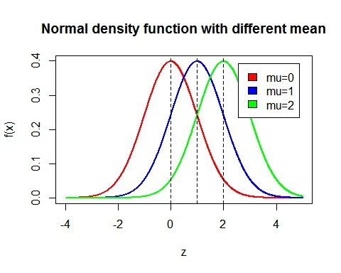
Notice how the curve shifts horizontally as the mean changes, but maintains the same shape.
Effect of Different Standard Deviations
Following is the graph of probability density function of normal distribution with the same mean ($\mu = 0$) while standard deviations differ ($\sigma = 1, 2, 3$):
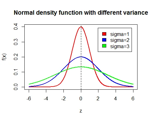
As the standard deviation increases, the curve becomes flatter and wider, indicating more variation in the data.
Cumulative Distribution Function (CDF)
The cumulative distribution function (CDF), denoted $F(x)$, gives the probability that $X$ is less than or equal to $x$:
$$ F(x) = P(X \leq x) = \int_{-\infty}^{x} f(t) , dt $$
For the normal distribution, this integral does not have a closed-form solution and is typically evaluated using standard normal tables or statistical software.
Key Properties of Normal Distribution
Mean of Normal Distribution
The mean of $N(\mu,\sigma^2)$ distribution is $E(X)=\mu$.
Proof
$$ \begin{eqnarray*} \text{Mean } &=& E(X) \ &=& \int_{-\infty}^\infty x f(x); dx\ &=& \frac{1}{\sigma\sqrt{2\pi}}\int_{-\infty}^\infty xe^{-\frac{1}{2\sigma^2}(x-\mu)^2} ; dx \end{eqnarray*} $$
Let $\dfrac{x-\mu}{\sigma}=z$ $\Rightarrow x=\mu+\sigma z$. Therefore, $dx = \sigma dz$.
$$ \begin{eqnarray*} \text{Mean } &=& \frac{1}{\sigma\sqrt{2\pi}}\int_{-\infty}^\infty (\mu+\sigma z)e^{-\frac{1}{2}z^2}\sigma ;dz\ &=& \frac{\mu }{\sqrt{2\pi}}\int_{-\infty}^\infty e^{-\frac{1}{2}z^2}; dz+\frac{1}{\sqrt{2\pi}}\int_{-\infty}^\infty ze^{-\frac{1}{2}z^2} ;dz\ &=& \frac{\mu }{\sqrt{2\pi}}\sqrt{2\pi} + 0 \quad (\text{second integral is odd function})\ &=& \mu \end{eqnarray*} $$
Variance of Normal Distribution
The variance of $N(\mu,\sigma^2)$ distribution is $V(X)=\sigma^2$.
Proof
$$ \begin{eqnarray*} \text{Variance } &=& E(X-\mu)^2 \ &=& \int_{-\infty}^\infty (x-\mu)^2 f(x); dx\ &=& \frac{1}{\sigma\sqrt{2\pi}}\int_{-\infty}^\infty (x-\mu)^2e^{-\frac{1}{2\sigma^2}(x-\mu)^2} ; dx \end{eqnarray*} $$
Using the substitution $z = \frac{x-\mu}{\sigma}$ and integration by parts:
$$ \text{Variance} = \sigma^2 $$
Standard Deviation
The standard deviation is $\sigma = \sqrt{V(X)} = \sqrt{\sigma^2} = \sigma$.
Additional Properties
| Property | Formula |
|---|---|
| Mean | $E(X) = \mu$ |
| Variance | $V(X) = \sigma^2$ |
| Standard Deviation | $\sigma$ |
| Median | $M = \mu$ |
| Mode | $Mo = \mu$ |
| Coefficient of Skewness | $\beta_1 = 0$ (symmetric) |
| Coefficient of Kurtosis | $\beta_2 = 3$ (mesokurtic) |
| Mean Deviation | $E[|X-\mu|] = \sqrt{\frac{2}{\pi}}\sigma$ |
Moment Generating Function (MGF)
The moment generating function of $N(\mu,\sigma^2)$ distribution is:
$$ M_X(t)=e^{t\mu +\frac{1}{2}t^2\sigma^2} $$
Proof
$$ \begin{eqnarray*} M_X(t) &=& E(e^{tX}) \ &=&\frac{1}{\sigma\sqrt{2\pi}}\int_{-\infty}^\infty e^{tx}e^{-\frac{1}{2\sigma^2}(x-\mu)^2} ; dx \end{eqnarray*} $$
Using the substitution $z = \frac{x-\mu}{\sigma}$ and completing the square:
$$ M_X(t) = e^{t\mu +\frac{1}{2}t^2\sigma^2} $$
Central Moments
All odd order central moments of $N(\mu,\sigma^2)$ distribution are 0:
$$\mu_1 = \mu_3 = \mu_5 = \cdots = 0$$
The $(2r)^{th}$ order central moment is:
$$\mu_{2r}= \frac{\sigma^{2r}(2r)!}{2^r (r)!}$$
This gives us:
- $\mu_2 = \sigma^2$ (variance)
- $\mu_4 = 3\sigma^4$
Skewness and Kurtosis
Coefficient of Skewness
$$\beta_1 = \frac{\mu_3^2}{\mu_2^3} = 0$$
The normal distribution is perfectly symmetric with no skew.
Coefficient of Kurtosis
$$\beta_2 = \frac{\mu_4}{\mu_2^2}= \frac{3\sigma^4}{\sigma^4}=3$$
The normal distribution is mesokurtic (medium-tailed).
Characteristics Function
The characteristics function of $N(\mu,\sigma^2)$ distribution is:
$$\phi_X(t)=e^{it\mu -\frac{1}{2}t^2\sigma^2}$$
Median and Mode
- Median: $M = \mu$
- Mode: $Mo = \mu$
For the normal distribution: mean = median = mode = $\mu$
This is a key characteristic of the symmetric normal distribution.
Empirical Rule (68-95-99.7 Rule)
For a normal distribution with mean $\mu$ and standard deviation $\sigma$:
-
68% of the data falls within one standard deviation of the mean: $P(\mu - \sigma < X < \mu + \sigma) \approx 0.68$
-
95% of the data falls within two standard deviations of the mean: $P(\mu - 2\sigma < X < \mu + 2\sigma) \approx 0.95$
-
99.7% of the data falls within three standard deviations of the mean: $P(\mu - 3\sigma < X < \mu + 3\sigma) \approx 0.997$
Standard Normal Distribution
If $X\sim N(\mu, \sigma^2)$ distribution, then the variate $Z =\frac{X-\mu}{\sigma}$ is called a standard normal variate and $Z\sim N(0,1)$ distribution.
The p.d.f. of standard normal variate $Z$ is:
$$ f(z)= \left{ \begin{array}{ll} \frac{1}{\sqrt{2\pi}}e^{-\frac{1}{2}z^2}, & \hbox{$-\infty < z<\infty$;} \ 0, & \hbox{Otherwise.} \end{array} \right. $$
Why Standardize?
Converting to standard normal distribution allows us to use standard normal tables and compare different normal distributions on the same scale.
Important Theorems
Sum of Independent Normal Variates
If $X \sim N(\mu_1, \sigma^2_1)$ and $Y \sim N(\mu_2, \sigma^2_2)$ are independent, then:
$$X+Y\sim N(\mu_1+\mu_2,\sigma^2_1+\sigma^2_2)$$
Difference of Independent Normal Variates
If $X \sim N(\mu_1, \sigma^2_1)$ and $Y \sim N(\mu_2, \sigma^2_2)$ are independent, then:
$$X-Y\sim N(\mu_1-\mu_2,\sigma^2_1+\sigma^2_2)$$
Distribution of Sample Mean
If $X_i, i=1,2,\cdots, n$ are independent observations from $N(\mu, \sigma^2)$ distribution, then:
$$\overline{X}\sim N\left(\mu,\frac{\sigma^2}{n}\right)$$
Examples with Solutions
Example 1: Heights of Men
Problem: A survey was conducted to measure the height of men in the 20-29 age group. Heights are normally distributed with mean $\mu = 69.8$ inches and standard deviation $\sigma = 2.1$ inches. A study participant is randomly selected.
a. Find the probability that his height is less than 66.5 inches. b. Find the probability that his height is between 65.5 and 71.6 inches. c. Find the probability that his height is more than 72.3 inches.
Solution:
Let $X$ denote the height of a randomly selected participant. Given: $X\sim N(69.8, 2.1^2)$
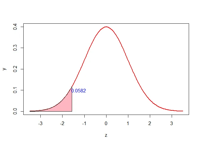
Part (a): $P(X < 66.5)$
First, convert to standard normal using $Z = \frac{X-\mu}{\sigma}$:
$$z = \frac{66.5-69.8}{2.1} = \frac{-3.3}{2.1} \approx -1.57$$
$$P(X < 66.5) = P(Z < -1.57) = 0.0582$$
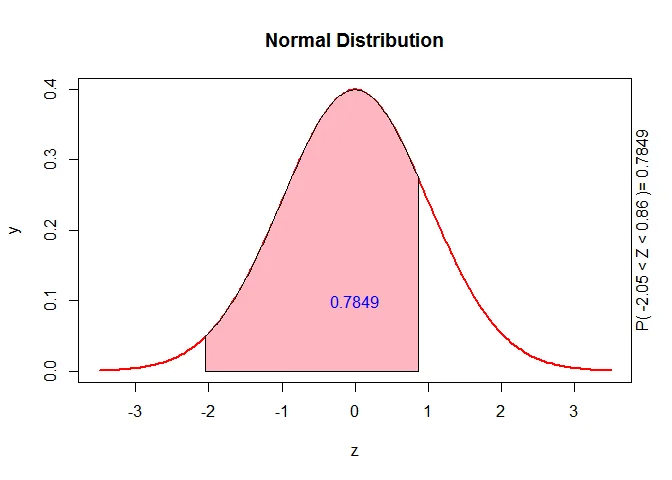
Part (b): $P(65.5 \leq X \leq 71.6)$
For $X = 65.5$: $$z_1 = \frac{65.5-69.8}{2.1} \approx -2.05$$
For $X = 71.6$: $$z_2 = \frac{71.6-69.8}{2.1} \approx 0.86$$
$$P(65.5 \leq X \leq 71.6) = P(-2.05 \leq Z \leq 0.86)$$ $$= P(Z < 0.86) - P(Z < -2.05)$$ $$= 0.8051 - 0.0202 = 0.7849$$
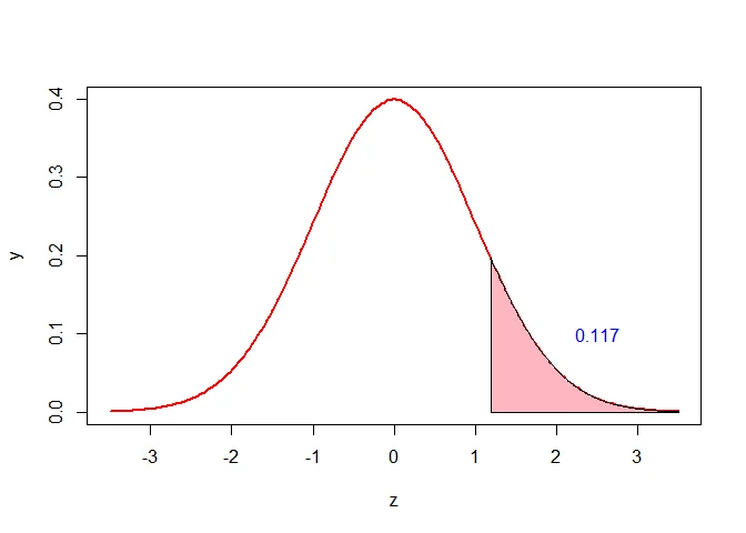
Part (c): $P(X > 72.3)$
$$z = \frac{72.3-69.8}{2.1} \approx 1.19$$
$$P(X > 72.3) = 1 - P(X \leq 72.3)$$ $$= 1 - P(Z \leq 1.19)$$ $$= 1 - 0.883 = 0.117$$
Example 2: College Grade Point Averages
Problem: The grade point averages of college students are approximately normally distributed with mean $\mu = 2.4$ and standard deviation $\sigma = 0.8$.
a. What percentage of students will have a GPA in excess of 3.0? b. What percentage of students will have a GPA less than 2.2? c. What percentage of students will have a GPA between 2.1 and 2.8?
Solution:
Let $X$ denote the GPA of college students. Given: $X\sim N(2.4, 0.8^2)$
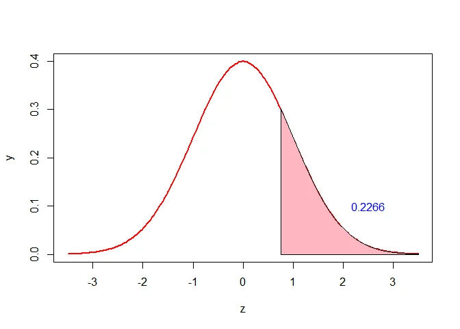
Part (a): $P(X > 3.0)$
$$z = \frac{3.0-2.4}{0.8} = 0.75$$
$$P(X > 3) = 1 - P(Z < 0.75) = 1 - 0.7734 = 0.2266$$
So 22.66% of students have a GPA exceeding 3.0.
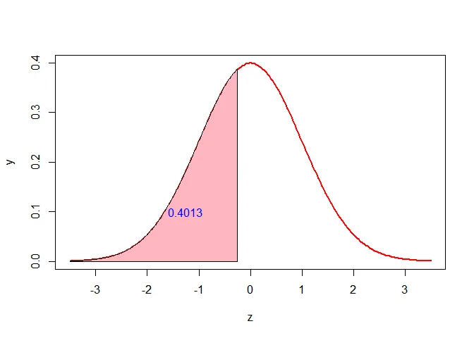
Part (b): $P(X < 2.2)$
$$z = \frac{2.2-2.4}{0.8} = -0.25$$
$$P(X < 2.2) = P(Z < -0.25) = 0.4013$$
So 40.13% of students have a GPA less than 2.2.
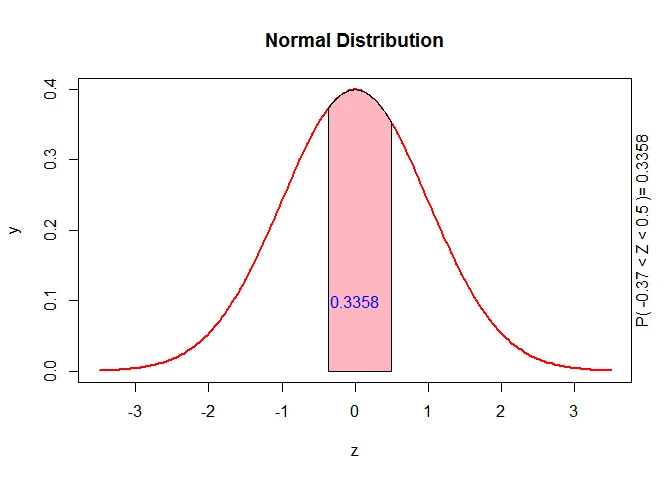
Part (c): $P(2.1 \leq X \leq 2.8)$
For $X = 2.1$: $$z_1 = \frac{2.1-2.4}{0.8} \approx -0.37$$
For $X = 2.8$: $$z_2 = \frac{2.8-2.4}{0.8} = 0.5$$
$$P(2.1 \leq X \leq 2.8) = P(-0.37 \leq Z \leq 0.5)$$ $$= P(Z < 0.5) - P(Z < -0.37)$$ $$= 0.6915 - 0.3557 = 0.3358$$
So 33.58% of students have a GPA between 2.1 and 2.8.
Properties Summary Table
| Property | Value |
|---|---|
| $f(x) = \frac{1}{\sigma\sqrt{2\pi}}e^{-\frac{1}{2\sigma^2}(x-\mu)^2}$ | |
| Support | $(-\infty, \infty)$ |
| Mean | $\mu$ |
| Median | $\mu$ |
| Mode | $\mu$ |
| Variance | $\sigma^2$ |
| Standard Deviation | $\sigma$ |
| Coefficient of Variation | $\frac{\sigma}{\mu}$ |
| Skewness | $0$ |
| Kurtosis | $3$ |
| MGF | $M_X(t) = e^{t\mu + \frac{1}{2}t^2\sigma^2}$ |
| CF | $\phi_X(t) = e^{it\mu - \frac{1}{2}t^2\sigma^2}$ |
| Entropy | $\frac{1}{2}\log(2\pi e\sigma^2)$ |
When to Use Normal Distribution
The normal distribution is appropriate when:
- Natural Measurements: Heights, weights, temperatures, and other natural measurements
- Sum of Many Variables: By the Central Limit Theorem, the sum or average of many independent random variables is approximately normal
- Symmetric Data: When data is roughly symmetric with no significant skew
- Quality Control: Manufacturing and quality control processes
- Financial Returns: Stock returns and other financial metrics (under certain conditions)
- Test Scores: Standardized test scores and exam results
- Experimental Measurements: Measurement errors and uncertainties in scientific experiments
Applications
- Risk Assessment: Used in financial modeling and insurance
- Quality Control: Monitoring product quality in manufacturing
- Hypothesis Testing: Foundation for many statistical tests
- Confidence Intervals: Constructing confidence intervals for population parameters
- Forecasting: Time series and regression analysis
- Medical Research: Analyzing medical measurements and treatment outcomes
- Engineering: Tolerance analysis and reliability engineering
Related Distributions
Related Continuous Distributions:
- Exponential Distribution - For right-skewed data
- Gamma Distribution - Generalizes exponential
- Weibull Distribution - For reliability analysis
- Log-Normal Distribution - Right-skewed alternative
Approximation Applications:
- Normal Approximation to Binomial - Discrete to continuous
- Normal Approximation to Poisson - Large-sample approximation
- Probability Distributions Complete Guide - Comprehensive reference
Connection to Other Distributions
- Central Limit Theorem: Any distribution with finite mean and variance will approximate a normal distribution when sample size is large
- Standard Normal (Z-distribution): Special case with $\mu = 0$ and $\sigma = 1$
- Log-normal: If $X$ is normal, then $e^X$ is log-normal
- t-distribution: Approximates normal for large sample sizes
- Chi-square Distribution: Sum of squared standard normals
References
-
Walpole, R.E., Myers, S.L., Myers, S.L., & Ye, K. (2012). Probability & Statistics for Engineers & Scientists (9th ed.). Pearson. - Comprehensive treatment of normal distribution, standard normal table, and Central Limit Theorem.
-
NIST/SEMATECH. (2023). e-Handbook of Statistical Methods. Retrieved from https://www.itl.nist.gov/div898/handbook/ - Normal distribution properties, applications, and relationship to other distributions.
Conclusion
The normal distribution is fundamental to statistics and widely used in real-world applications. Its mathematical properties make it ideal for theoretical analysis and its appearance in natural phenomena makes it practically important. Understanding the normal distribution;its properties, parameters, and applications;is essential for anyone working with statistics or data analysis.
The ability to standardize normal random variables, use standard normal tables, and apply the empirical rule makes the normal distribution accessible and powerful for solving practical problems in science, engineering, business, and research.