Poisson Distribution
The Poisson distribution is one of the most important discrete probability distributions in statistics. It helps describe the probability of occurrence of a number of events in some given time interval or in a specified region. The time interval may be of any length, such as minutes, days, or weeks.
Definition of Poisson Distribution
A discrete random variable $X$ is said to have Poisson distribution with parameter $\lambda$ if its probability mass function is
$$ \begin{equation*} P(X=x)= \left\{ \begin{array}{ll} \frac{e^{-\lambda}\lambda^x}{x!} , & \hbox{$x=0,1,2,\cdots; \lambda>0$;} \\ 0, & \hbox{Otherwise.} \end{array} \right. \end{equation*} $$
The variate $X$ is called Poisson variate and $\lambda$ is called the parameter of Poisson distribution.
In notation, it can be written as $X\sim P(\lambda)$.
Key Features of Poisson Distribution
- Let $X$ denote the number of times an event occurs in a given interval. The interval can be time, area, volume, or distance.
- The probability of occurrence of an event is the same for each interval.
- The occurrence of an event in one interval is independent of the occurrence in other intervals.
Poisson Distribution as a Limiting Form of Binomial Distribution
In binomial distribution, if $n\to \infty$, $p\to 0$ such that $np=\lambda$ (finite), then binomial distribution tends to Poisson distribution.
Proof
Let $X\sim B(n,p)$ distribution. Then the probability mass function of $X$ is
$$ \begin{equation*} P(X=x)= \left\{ \begin{array}{ll} \binom{n}{x} p^x q^{n-x}, & \hbox{$x=0,1,2,\cdots, n; 0<p<1; q=1-p$} \\ 0, & \hbox{Otherwise.} \end{array} \right. \end{equation*} $$
Taking the $\lim$ as $n\to \infty$ and $p\to 0$, we have
$$ \begin{eqnarray*} P(x) &=& \lim_{n\to\infty \atop{p\to 0}} \binom{n}{x} p^x q^{n-x} \\ &=& \lim_{n\to\infty \atop{p\to 0}} \frac{n!}{(n-x)!x!} p^x q^{n-x} \\ &=& \lim_{n\to\infty \atop{p\to 0}} \frac{n(n-1)(n-2)\cdots (n-x+1)}{x!} p^x q^{n-x} \\ &=& \lim_{n\to\infty \atop{p\to 0}} \frac{n^x(-\frac{1}{n})(1-\frac{2}{n})\cdots (1-\frac{x-1}{n})}{x!} p^x (1-p)^{n-x} \\ &=& \lim_{n\to\infty \atop{p\to 0}} \frac{(np)^x(1-\frac{1}{n})(1-\frac{2}{n})\cdots (1-\frac{x-1}{n})}{x!}(1-p)^{n-x} \\ &=& \lim_{n\to\infty \atop{p\to 0}} \frac{\lambda^x}{x!}\big(1-\frac{1}{n}\big)\big(1-\frac{2}{n}\big)\cdots \big(1-\frac{x-1}{n}\big)\big(1-\frac{\lambda}{n}\big)^{n-x} \\ &=& \frac{\lambda^x}{x!}\lim_{n\to\infty }\bigg[\big(1-\frac{\lambda}{n}\big)^{-n/\lambda}\bigg]^{-\lambda}\big(1-\frac{\lambda}{n}\big)^{-x} \\ &=& \frac{\lambda^x}{x!}e^{-\lambda} (1)^{-x}\qquad (\because \lim_{n\to \infty}\big(1-\frac{\lambda}{n}\big)^{-n/\lambda}=e)\\ &=& \frac{e^{-\lambda}\lambda^x}{x!},\;\; x=0,1,2,\cdots; \lambda>0. \end{eqnarray*} $$
Clearly, $P(x)\geq 0$ for all $x\geq 0$, and
$$ \begin{eqnarray*} \sum_{x=0}^\infty P(x) &=& \sum_{x=0}^\infty \frac{e^{-\lambda}\lambda^x}{x!} \\ &=& e^{-\lambda}\sum_{x=0}^\infty \frac{\lambda^x}{x!} \\ &=& e^{-\lambda}\bigg(1+\frac{\lambda}{1!}+\frac{\lambda^2}{2!}+\cdots + \bigg)\\ &=& e^{-\lambda}e^{\lambda}=1. \end{eqnarray*} $$
Hence, $P(x)$ is a legitimate probability mass function.
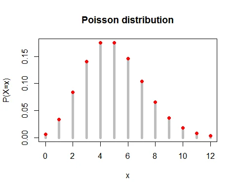
Graph of Poisson Distribution
Following graph shows the probability mass function of Poisson distribution with parameter $\lambda = 5$.
Mean of Poisson Distribution
The expected value of Poisson random variable is $E(X)=\lambda$.
Proof
The expected value of Poisson random variable is
$$ \begin{eqnarray*} E(X) &=& \sum_{x=0}^\infty x\cdot P(X=x)\\ &=& \sum_{x=0}^\infty x\cdot \frac{e^{-\lambda}\lambda^x}{x!}\\ &=& 0 +\lambda e^{-\lambda}\sum_{x=1}^\infty \frac{\lambda^{x-1}}{(x-1)!}\\ &=& \lambda e^{-\lambda}\bigg(1+\frac{\lambda}{1!}+\frac{\lambda^2}{2!}+\cdots + \bigg)\\ &=& \lambda e^{-\lambda}e^{\lambda} \\ &=& \lambda. \end{eqnarray*} $$
Variance of Poisson Distribution
The variance of Poisson random variable is $V(X) =\lambda$.
Proof
The variance of random variable $X$ is given by
$$ V(X) = E(X^2) - [E(X)]^2 $$
Let us find the expected value $X^2$.
$$ \begin{eqnarray*} E(X^2) & = & E[X(X-1)]+ E(X)\\ &=& \sum_{x=0}^\infty x(x-1)\cdot P(X=x)+\lambda\\ &=& \sum_{x=0}^\infty x(x-1)\cdot \frac{e^{-\lambda}\lambda^x}{x!} +\lambda\\ &=& 0 +0+\lambda^2 e^{-\lambda}\sum_{x=2}^\infty \frac{\lambda^{x-2}}{(x-2)!}+\lambda\\ &=& \lambda^2 e^{-\lambda}\bigg(1+\frac{\lambda}{1!}+\frac{\lambda^2}{2!}+\cdots + \bigg)+\lambda\\ &=& \lambda^2 e^{-\lambda}e^{\lambda} = \lambda^2+\lambda. \end{eqnarray*} $$
Thus, variance of Poisson random variable is
$$ \begin{eqnarray*} V(X) &=& E(X^2) - [E(X)]^2\\ &=& \lambda^2+\lambda-\lambda^2\\ &=& \lambda. \end{eqnarray*} $$
Key Property: For Poisson distribution, Mean = Variance = $\lambda$.
Moment Generating Function of Poisson Distribution
The moment generating function of Poisson distribution is $M_X(t)=e^{\lambda(e^t-1)}, t \in R$.
Proof
The moment generating function of Poisson random variable $X$ is
$$ \begin{eqnarray*} M_X(t) &=& E(e^{tx}) \\ &=& \sum_{x=0}^\infty e^{tx} \frac{e^{-\lambda}\lambda^x}{x!}\\ &=& e^{-\lambda}\sum_{x=0}^\infty \frac{(\lambda e^{t})^x}{x!}\\ &=& e^{-\lambda}\cdot e^{\lambda e^t}\\ &=& e^{\lambda(e^t-1)}, \; t\in R. \end{eqnarray*} $$
Moments from MGF
The $r^{th}$ moment of Poisson random variable is given by
$$ \begin{equation*} \mu_r^\prime=\bigg[\frac{d^r M_X(t)}{dt^r}\bigg]_{t=0}. \end{equation*} $$
Proof
The moment generating function of Poisson distribution is $M_X(t) =e^{\lambda(e^t-1)}$.
Differentiating $M_X(t)$ with respect to $t$:
$$ \begin{equation} \frac{d M_X(t)}{dt}= e^{\lambda(e^t-1)}(\lambda e^{t}). \end{equation} $$
Putting $t=0$:
$$ \begin{eqnarray*} \mu_1^\prime &=& \bigg[\frac{d M_X(t)}{dt}\bigg]_{t=0} \\ &=& \bigg[e^{\lambda(e^t-1)}(\lambda e^{t})\bigg]_{t=0}\\ &=& \lambda = \text{ mean }. \end{eqnarray*} $$
Again differentiating with respect to $t$:
$$ \begin{equation*} \frac{d^2 M_X(t)}{dt^2}= e^{\lambda(e^t-1)}(\lambda e^{t})+(\lambda e^t)e^{\lambda(e^t-1)}(\lambda e^{t}). \end{equation*} $$
Putting $t=0$:
$$ \begin{eqnarray*} \mu_2^\prime &=& \bigg[\frac{d^2 M_X(t)}{dt^2}\bigg]_{t=0} \\ &=& \lambda+\lambda^2. \end{eqnarray*} $$
Hence, variance $= \mu_2 = \mu_2^\prime - (\mu_1^\prime)^2=\lambda+\lambda^2-\lambda^2=\lambda$.
Characteristics Function of Poisson Distribution
The characteristics function of Poisson distribution is $\phi_X(t)=e^{\lambda(e^{it}-1)}, t \in R$.
Proof
The characteristics function of Poisson random variable $X$ is
$$ \begin{eqnarray*} \phi_X(t) &=& E(e^{itx}) \\ &=& \sum_{x=0}^\infty e^{itx} \frac{e^{-\lambda}\lambda^x}{x!}\\ &=& e^{-\lambda}\sum_{x=0}^\infty \frac{(\lambda e^{it})^x}{x!}\\ &=& e^{-\lambda}\cdot e^{\lambda e^{it}}\\ &=& e^{\lambda(e^{it}-1)}, \; t\in R. \end{eqnarray*} $$
Probability Generating Function
The probability generating function of Poisson distribution is $P_X(t)=e^{\lambda(t-1)}$.
Proof
Let $X\sim P(\lambda)$ distribution. Then the p.g.f. of $X$ is
$$ \begin{eqnarray*} P_X(t) &=& E(t^x) \\ &=& \sum_{x=0}^\infty t^x \frac{e^{-\lambda}\lambda^x}{x!}\\ &=& e^{-\lambda}\sum_{x=0}^\infty \frac{(\lambda t)^x}{x!}\\ &=& e^{-\lambda}\cdot e^{\lambda t}\\ &=& e^{\lambda(t-1)}. \end{eqnarray*} $$
Additive Property of Poisson Distribution
The sum of two independent Poisson variates is also a Poisson variate.
If $X_1$ and $X_2$ are two independent Poisson variates with parameters $\lambda_1$ and $\lambda_2$ respectively, then $X_1+X_2 \sim P(\lambda_1+\lambda_2)$.
Proof
Let $X_1$ and $X_2$ be two independent Poisson variates with parameters $\lambda_1$ and $\lambda_2$ respectively.
Then the MGF of $X_1$ is $M_{X_1}(t) =e^{\lambda_1(e^t-1)}$ and the MGF of $X_2$ is $M_{X_2}(t) =e^{\lambda_2(e^t-1)}$.
Let $Y=X_1+X_2$. Then the MGF of $Y$ is
$$ \begin{eqnarray*} M_Y(t) &=& E(e^{tY}) \\ &=& E(e^{t(X_1+X_2)}) \\ &=& E(e^{tX_1} e^{tX_2}) \\ &=& E(e^{tX_1})\cdot E(e^{tX_2})\\ & & \quad \qquad (\because X_1, X_2 \text{ are independent })\\ &=& M_{X_1}(t)\cdot M_{X_2}(t)\\ &=& e^{\lambda_1(e^t-1)}\cdot e^{\lambda_2(e^t-1)}\\ &=& e^{(\lambda_1+\lambda_2)(e^t-1)}. \end{eqnarray*} $$
which is the m.g.f. of Poisson variate with parameter $\lambda_1+\lambda_2$.
Hence, by uniqueness theorem of MGF, $Y=X_1+X_2$ follows a Poisson distribution with parameter $\lambda_1+\lambda_2$.
Mode of Poisson Distribution
The condition for mode of Poisson distribution is $\lambda-1 \leq x\leq \lambda$.
Proof
The mode is that value of $x$ for which $P(x)$ is greater than or equal to $P(x-1)$ and $P(x+1)$, i.e., $P(x-1)\leq P(x) \geq P(x+1)$.
Now, $P(x-1)\leq P(x)$ gives
$$ \begin{eqnarray*} \frac{e^{-\lambda}\lambda^{(x-1)}}{(x-1)!} &\leq& \frac{e^{-\lambda}\lambda^{x}}{x!} \\ x &\leq & \lambda. \end{eqnarray*} $$
And $P(x) \geq P(x+1)$ gives
$$ \begin{eqnarray*} \frac{e^{-\lambda}\lambda^{x}}{x!} &\leq& \frac{e^{-\lambda}\lambda^{(x+1)}}{(x+1)!} \\ \lambda-1 &\leq & x. \end{eqnarray*} $$
Hence, the condition for mode of Poisson distribution is $\lambda-1 \leq x\leq \lambda$.
Recurrence Relations
Recurrence Relation for Raw Moments
The recurrence relation for raw moments of Poisson distribution is
$$ \begin{equation*} \mu_{r+1}^\prime = \lambda \bigg[ \frac{d\mu_r^\prime}{d\lambda} + \mu_r^\prime\bigg]. \end{equation*} $$
Recurrence Relation for Central Moments
The recurrence relation for central moments of Poisson distribution is
$$ \begin{equation*} \mu_{r+1} = \lambda \bigg[ \frac{d\mu_r}{d\lambda} + r\mu_{r-1}\bigg]. \end{equation*} $$
Recurrence Relation for Probabilities
The recurrence relation for probabilities of Poisson distribution is
$$ \begin{equation*} P(X=x+1) = \frac{\lambda}{x+1}\cdot P(X=x), \; x=0,1,2\cdots. \end{equation*} $$
Poisson Distribution Examples
Example 1: Typing Errors in a Book
A book contains 500 pages. If there are 200 typing errors randomly distributed throughout the book, use the Poisson distribution to determine the probability that a page contains:
a. exactly 3 errors b. at least 3 errors c. at most 2 errors d. 2 or more errors but less than 5 errors
Solution
The average number of typing errors per page: $\lambda =\frac{200}{500}= 0.4$.
The random variable $X$ is the number of typing errors per page, $X\sim P(0.4)$.
The probability mass function is:
$$ \begin{aligned} P(X=x) &= \frac{e^{-0.4}(0.4)^x}{x!},\; x=0,1,2,\cdots \end{aligned} $$
a. Exactly 3 errors:
$$ \begin{aligned} P(X=3) &= \frac{e^{-0.4}0.4^{3}}{3!}\\ &= 0.0072 \end{aligned} $$
b. At least 3 errors:
$$ \begin{aligned} P(X\geq3) &= 1- P(X\leq 2)\\ &= 1- \sum_{x=0}^{2}P(X=x)\\ &= 1- \big[P(X=0) + P(X=1) + P(X=2)\big]\\ &= 1- \bigg[ \frac{e^{-0.4}0.4^{0}}{0!}+ \frac{e^{-0.4}0.4^{1}}{1!}+ \frac{e^{-0.4}0.4^{2}}{2!}\bigg]\\ &= 1-\big(0.6703+0.2681+0.0536\big)\\ &= 1-0.992\\ &= 0.008 \end{aligned} $$
c. At most 2 errors:
$$ \begin{aligned} P(X\leq2) &= \sum_{x=0}^{2}P(X=x)\\ &= P(X=0) + P(X=1) + P(X=2)\\ &= \frac{e^{-0.4}0.4^{0}}{0!}+ \frac{e^{-0.4}0.4^{1}}{1!}+ \frac{e^{-0.4}0.4^{2}}{2!}\\ &= 0.6703+0.2681+0.0536\\ &= 0.992 \end{aligned} $$
d. 2 or more but less than 5 errors:
$$ \begin{aligned} P(2\leq X< 5) &=P(2\leq X\leq 4)\\ &=P(X=2)+P(X=3)+P(X=4)\\ &= \frac{e^{-0.4}0.4^{2}}{2!}+\frac{e^{-0.4}0.4^{3}}{3!}+\frac{e^{-0.4}0.4^{4}}{4!}\\ &= 0.0536+0.0072+0.0007\\ &= 0.0615 \end{aligned} $$
Example 2: Traffic Accidents
Suppose that in a certain area there are on average 5 traffic accidents per month. Find the probability of:
a. 4 accidents in a given month b. at least 2 accidents in a given month c. at most 2 accidents in a given month
Solution
The average number of traffic accidents per month: $\lambda = 5$.
The random variable $X$ is the number of traffic accidents per month, $X\sim P(5)$.
The probability mass function is:
$$ \begin{aligned} P(X=x) &= \frac{e^{-5}(5)^x}{x!},\; x=0,1,2,\cdots \end{aligned} $$
a. 4 accidents in a given month:
$$ \begin{aligned} P(X=4) &= \frac{e^{-5}5^{4}}{4!}\\ &= 0.1755 \end{aligned} $$
b. At least 2 accidents:
$$ \begin{aligned} P(X\geq2) &= 1- P(X\leq 1)\\ &= 1- \sum_{x=0}^{1}P(X=x)\\ &= 1- \big[P(X=0) + P(X=1)\big]\\ &= 1- \bigg[ \frac{e^{-5}5^{0}}{0!}+ \frac{e^{-5}5^{1}}{1!}\bigg]\\ &= 1-\big(0.0067+0.0337\big)\\ &= 1-0.0404\\ &= 0.9596 \end{aligned} $$
c. At most 2 accidents:
$$ \begin{aligned} P(X\leq2) &= \sum_{x=0}^{2}P(X=x)\\ &= P(X=0) + P(X=1) + P(X=2)\\ &= \frac{e^{-5}5^{0}}{0!}+ \frac{e^{-5}5^{1}}{1!}+ \frac{e^{-5}5^{2}}{2!}\\ &= 0.0067+0.0337+0.0842\\ &= 0.1246 \end{aligned} $$
Properties Summary Table
| Property | Formula |
|---|---|
| PMF | $P(X=x) = \frac{e^{-\lambda}\lambda^x}{x!}$ |
| Mean | $E(X) = \lambda$ |
| Variance | $V(X) = \lambda$ |
| Standard Deviation | $\sigma = \sqrt{\lambda}$ |
| MGF | $M_X(t) = e^{\lambda(e^t-1)}$ |
| PGF | $P_X(t) = e^{\lambda(t-1)}$ |
| Mode | $\lambda - 1 \leq x \leq \lambda$ |
When to Use Poisson Distribution
The Poisson distribution is appropriate when:
- You are counting the number of events occurring in a fixed interval (time, distance, area, or volume)
- Events occur independently
- The average rate of events is constant
- Two events cannot occur at exactly the same instant
- The number of events in one interval is independent of the number in other intervals
Common Applications:
- Number of customer arrivals at a service desk per hour
- Number of defects in manufactured items
- Number of phone calls received at a switchboard per minute
- Number of traffic accidents on a highway per day
- Number of spelling errors in a page of a book
- Number of radioactive particles emitted per time interval
- Number of disease cases in a population per time period
Related Distributions
Similar Discrete Distributions:
- Binomial Distribution - Fixed trials with two outcomes
- Exponential Distribution - Continuous waiting time analog
- Geometric Distribution - Trials until first success
- Negative Binomial Distribution - Trials until r successes
Approximation Theorems:
- Poisson Approximation to Binomial - When to use Poisson for Binomial
- Normal Approximation to Poisson - Approximation for large λ
References
-
Anderson, D.R., Sweeney, D.J., & Williams, T.A. (2018). Statistics for Business and Economics (14th ed.). Cengage Learning. - Poisson distribution for modeling rare events and counting processes in business contexts.
-
NIST/SEMATECH. (2023). e-Handbook of Statistical Methods. Retrieved from https://www.itl.nist.gov/div898/handbook/ - Technical specifications and properties of Poisson distribution with practical applications.
Conclusion
The Poisson distribution is a fundamental tool in probability theory and statistics with wide-ranging practical applications. Its simple structure, where mean equals variance, makes it particularly useful for modeling rare events and count data in various fields including quality control, telecommunications, and epidemiology.