Testing Significance of Linear Relationship
A test of significance for a linear relationship between the variables $x$ and $y$ can be performed using the sample correlation coefficient $r_{xy}$.
Example 1
For a sample of eight bears, researchers measured the distances around the bears’ chests and weighed the bears. The Sample correlation coefficient between the chest size and weight of bears is $r=0.744$ for $n=8$ bears. Using $\alpha=0.05$, determine if there is a positive linear correlation between chest size and weight.
Solution
Given that $n = 8$ pair of observations, sample correlation coefficient is $r= 0.744$.
Step 1 Hypothesis Testing Problem
The hypothesis testing problem is $H_0 : \rho = 0$ against $H_1 : \rho > 0$ ($\text{right-tailed}$)
Step 2 Test Statistic
The test statistic is
$$ \begin{aligned} t& =\frac{r}{\sqrt{1-r^2}}\sqrt{n-2} \end{aligned} $$
which follows $t$ distribution with $n-2$ degrees of freedom.
Step 3 Significance Level
The significance level is $\alpha = 0.05$.
Step 4 Critical Value(s)
As the alternative hypothesis is $\text{right-tailed}$, the critical value of $t$ $\text{is}$ $1.943$.
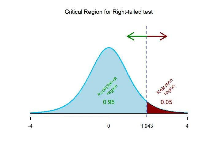
The rejection region (i.e. critical region) is $\text{t > 1.943}$.
Step 5 Computation
The test statistic under the null hypothesis is
$$ \begin{aligned} t&=\frac{r}{\sqrt{1-r^2}}\sqrt{n-2}\\ &= \frac{0.744}{\sqrt{1-0.744^2}}\sqrt{8 -2}\\ &= 2.727 \end{aligned} $$
Step 6 Decision (Traditional Approach)
The test statistic is $t =2.727$ which falls $\text{inside}$ the critical region, we $\text{reject}$ the null hypothesis.
OR
Step 6 Decision ($p$-value Approach)
This is a $\text{right-tailed}$ test, so the p-value is the area to the right of the test statistic ($t=2.727$) is p-value = $0.0172$.
The p-value is $0.0172$ which is $\text{less than}$ the significance level of $\alpha = 0.05$, we $\text{reject}$ the null hypothesis.
Interpretation
There is sufficient evidence to conclude that there is a significant positive linear relationship between chest size and weight of bears.
Example 2
Following is the data about the demand and price of a commodity for 8 periods.
| Demand | 16 | 20 | 18 | 21 | 13 | 15 | 17 | 22 |
|---|---|---|---|---|---|---|---|---|
| Price | 10 | 8 | 12 | 6 | 13 | 9 | 11 | 7 |
It was expected to estimate a linear regression for demand and price of a commodity.
Test whether there is a significant negative relationship between price and demand of a product.
Solution
Let $x$ denote the price of a commodity and $y$ denote the demand of a commodity.
The number of pairs $n= 8$.
| $x$ | $y$ | $x^2$ | $y^2$ | $xy$ | |
|---|---|---|---|---|---|
| 1 | 10 | 16 | 100 | 256 | 160 |
| 2 | 8 | 20 | 64 | 400 | 160 |
| 3 | 12 | 18 | 144 | 324 | 216 |
| 4 | 6 | 21 | 36 | 441 | 126 |
| 5 | 13 | 13 | 169 | 169 | 169 |
| 6 | 9 | 15 | 81 | 225 | 135 |
| 7 | 11 | 17 | 121 | 289 | 187 |
| 8 | 7 | 22 | 49 | 484 | 154 |
| Total | 76 | 142 | 764 | 2588 | 1307 |
The sample variance of $x$ is
$$ \begin{aligned} s_{x}^2 & = \frac{1}{n-1}\bigg(\sum x^2 - \frac{(\sum x)^2}{n}\bigg)\\ & = \frac{1}{8-1}\bigg(764-\frac{(76)^2}{8}\bigg)\\ &= \frac{1}{7}\bigg(764-\frac{5776}{8}\bigg)\\ &= \frac{1}{7}\bigg(764-722\bigg)\\ &= \frac{42}{7}\\ &= 6. \end{aligned} $$
The sample variance of $x$ is
$$ \begin{aligned} s_{y}^2 & = \frac{1}{n-1}\bigg(\sum y^2 - \frac{(\sum y)^2}{n}\bigg)\\ & = \frac{1}{8-1}\bigg(2588-\frac{(142)^2}{8}\bigg)\\ &= \frac{1}{7}\bigg(2588-\frac{20164}{8}\bigg)\\ &= \frac{1}{7}\bigg(2588-2520.5\bigg)\\ &= \frac{67.5}{7}\\ &= 9.6429. \end{aligned} $$
The sample covariance between $x$ and $y$ is
$$ \begin{aligned} s_{xy} & = \frac{1}{n-1}\bigg(\sum xy - \frac{(\sum x)(\sum y)}{n}\bigg)\\ & = \frac{1}{8-1}\bigg(1307-\frac{(76)(142)}{8}\bigg)\\ &= \frac{1}{7}\bigg(1307-\frac{10792}{8}\bigg)\\ &= \frac{1}{7}\bigg(1307-1349\bigg)\\ &= \frac{-42}{7}\\ &= -6. \end{aligned} $$
The Karl Pearson’s sample correlation coefficient between price of a commodity and demand of a commodity is
$$ \begin{aligned} r_{xy} & = \frac{Cov(x,y)}{\sqrt{V(x) V(y)}}\\ &= \frac{s_{xy}}{\sqrt{s_x^2s_y^2}}\\ &=\frac{-6}{\sqrt{6\times 9.6429}}\\ &=\frac{-6}{\sqrt{57.8574}}\\ &=-0.789. \end{aligned} $$
The correlation coefficient between price of a commodity and demand of a commodity is $-0.789$.
Step 1 Hypothesis Testing Problem
The hypothesis testing problem is $H_0 : \rho = 0$ against $H_1 : \rho < 0$ ($\text{left-tailed}$)
Step 2 Test Statistic
The test statistic is
$$ \begin{aligned} t& =\frac{r}{\sqrt{1-r^2}}\sqrt{n-2} \end{aligned} $$
which follows $t$ distribution with $n-2$ degrees of freedom.
Step 3 Significance Level
The significance level is $\alpha = 0.05$.
Step 4 Critical Value(s)
As the alternative hypothesis is $\text{left-tailed}$, the critical value of $t$ $\text{is}$ $-1.943$.
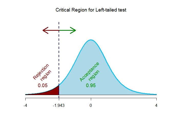
The rejection region (i.e. critical region) is $\text{t < -1.943}$.
Step 5 Computation
The test statistic under the null hypothesis is
$$ \begin{aligned} t&=\frac{r}{\sqrt{1-r^2}}\sqrt{n-2}\\ &= \frac{-0.789}{\sqrt{1--0.789^2}}\sqrt{8 -2}\\ &= -3.146 \end{aligned} $$
Step 6 Decision (Traditional Approach)
The test statistic is $t =-3.146$ which falls $\text{inside}$ the critical region, we $\text{reject}$ the null hypothesis.
OR
Step 6 Decision ($p$-value Approach)
This is a $\text{left-tailed}$ test, so the p-value is the area to the left of the test statistic ($t=-3.146$) is p-value = $0.01$.
The p-value is $0.01$ which is $\text{less than}$ the significance level of $\alpha = 0.05$, we $\text{reject}$ the null hypothesis.
Interpretation
There is sufficient evidence to conclude that there is a significant negative linear relationship between demand and price of a commodity.
Example 3
Following is the data about the exam scores of 10 randomly selected students and the number of hours they studied for the exam.
| Hours studied | 4 | 5 | 6 | 9 | 10 | 8 | 7 | 3 | 8 | 5 |
|---|---|---|---|---|---|---|---|---|---|---|
| Exam score | 68 | 65 | 85 | 84 | 82 | 86 | 83 | 76 | 67 | 74 |
Test whether there is a significant correlation between hours studied and examination score. Use $\alpha=0.01$.
Solution
Let $x$ denote the hours studied and $y$ denote the exam score.
The number of pairs $n= 11$.
| $x$ | $y$ | $x^2$ | $y^2$ | $xy$ | |
|---|---|---|---|---|---|
| 1 | 4 | 68 | 16 | 4624 | 272 |
| 2 | 5 | 65 | 25 | 4225 | 325 |
| 3 | 6 | 85 | 36 | 7225 | 510 |
| 4 | 9 | 84 | 81 | 7056 | 756 |
| 5 | 10 | 62 | 100 | 3844 | 620 |
| 6 | 8 | 86 | 64 | 7396 | 688 |
| 7 | 10 | 83 | 100 | 6889 | 830 |
| 8 | 7 | 76 | 49 | 5776 | 532 |
| 9 | 3 | 67 | 9 | 4489 | 201 |
| 10 | 8 | 74 | 64 | 5476 | 592 |
| 11 | 5 | 69 | 25 | 4761 | 345 |
| Total | 75 | 819 | 569 | 61761 | 5671 |
The sample variance of $x$ is
$$ \begin{aligned} s_{x}^2 & = \frac{1}{n-1}\bigg(\sum x^2 - \frac{(\sum x)^2}{n}\bigg)\\ & = \frac{1}{11-1}\bigg(569-\frac{(75)^2}{11}\bigg)\\ &= \frac{1}{10}\bigg(569-\frac{5625}{11}\bigg)\\ &= \frac{1}{10}\bigg(569-511.3636\bigg)\\ &= \frac{57.6364}{10}\\ &= 5.7636. \end{aligned} $$
The sample variance of $x$ is
$$ \begin{aligned} s_{y}^2 & = \frac{1}{n-1}\bigg(\sum y^2 - \frac{(\sum y)^2}{n}\bigg)\\ & = \frac{1}{11-1}\bigg(61761-\frac{(819)^2}{11}\bigg)\\ &= \frac{1}{10}\bigg(61761-\frac{670761}{11}\bigg)\\ &= \frac{1}{10}\bigg(61761-60978.2727\bigg)\\ &= \frac{782.7273}{10}\\ &= 78.2727. \end{aligned} $$
The sample covariance between $x$ and $y$ is
$$ \begin{aligned} s_{xy} & = \frac{1}{n-1}\bigg(\sum xy - \frac{(\sum x)(\sum y)}{n}\bigg)\\ & = \frac{1}{11-1}\bigg(5671-\frac{(75)(819)}{11}\bigg)\\ &= \frac{1}{10}\bigg(5671-\frac{61425}{11}\bigg)\\ &= \frac{1}{10}\bigg(5671-5584.0909\bigg)\\ &= \frac{86.9091}{10}\\ &= 8.6909. \end{aligned} $$
The Karl Pearson’s sample correlation coefficient between hours studied and exam score is
$$ \begin{aligned} r_{xy} & = \frac{Cov(x,y)}{\sqrt{V(x) V(y)}}\\ &= \frac{s_{xy}}{\sqrt{s_x^2s_y^2}}\\ &=\frac{8.6909}{\sqrt{5.7636\times 78.2727}}\\ &=\frac{8.6909}{\sqrt{451.1325}}\\ &=0.409. \end{aligned} $$
The sample correlation coefficient between hours studied and exam score is $0.409$.
Step 1 Hypothesis Testing Problem
The hypothesis testing problem is $H_0 : \rho = 0$ against $H_1 : \rho \neq 0$ ($\text{two-tailed}$)
Step 2 Test Statistic
The test statistic is
$$ \begin{aligned} t& =\frac{r}{\sqrt{1-r^2}}\sqrt{n-2} \end{aligned} $$
which follows $t$ distribution with $n-2$ degrees of freedom.
Step 3 Significance Level
The significance level is $\alpha = 0.01$.
Step 4 Critical Value(s)
As the alternative hypothesis is $\text{two-tailed}$, the critical value of $t$ $\text{are}$ $-3.25 and 3.25$.
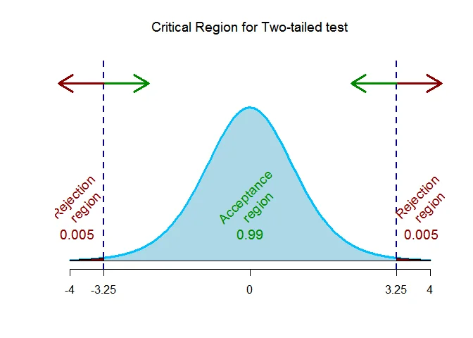
The rejection region (i.e. critical region) is $\text{t < -3.25 or t > 3.25}$.
Step 5 Computation
The test statistic under the null hypothesis is
$$ \begin{aligned} t&=\frac{r}{\sqrt{1-r^2}}\sqrt{n-2}\\ &= \frac{0.409}{\sqrt{1-0.409^2}}\sqrt{11 -2}\\ &= 1.345 \end{aligned} $$
Step 6 Decision (Traditional Approach)
The test statistic is $t =1.345$ which falls $\text{outside}$ the critical region, we $\text{fail to reject}$ the null hypothesis.
OR
Step 6 Decision ($p$-value Approach)
This is a $\text{two-tailed}$ test, so the p-value is the twice the area to the right of the test statistic ($t=1.345$) is p-value = $0.2117$.
The p-value is $0.2117$ which is $\text{greater than}$ the significance level of $\alpha = 0.01$, we $\text{fail to reject}$ the null hypothesis.
Interpretation
There is insufficient evidence to conclude that there is a significant linear relationship between hours studied and examination score because the correlation coefficient between $x$ and $y$ is not significantly different from zero.