Hypergeometric Distribution

Hypergeometric Experiment

A hypergeometric experiment is an experiment which satisfies each of the following conditions:

• The population or set to be sampled consists of $N$ individuals, objects, or elements (a finite population).
• Each object can be characterized as a “defective” or “non-defective”, and there are $M$ defectives in the population.
• A sample of $n$ individuals is drawn in such a way that each subset of size $n$ is equally likely to be chosen.

Hypergeometric Distribution

Suppose we have an hypergeometric experiment. That is, suppose there are $N$ units in the population and $M$ out of $N$ are defective, so $N-M$ units are non-defective.

Let $X$ denote the number of defective in a completely random sample of size $n$ drawn from a population consisting of total $N$ units.

The total number of ways of finding $n$ units out of $N$ is $\binom{N}{n}$. Out of $M$ defective units $x$ defective units can be selected in $\binom{M}{x}$ ways and out of $N-M$ non-defective units remaining $(n-x)$ units can be selected in $\binom{N-M}{n-x}$ ways.

Hence, probability of selecting $x$ defective units in a random sample of $n$ units out of $N$ is $$\begin{equation*} P(X=x) =\frac{\text{Favourable Cases}}{\text{Total Cases}} \end{equation*}$$

$$\begin{equation*} \therefore P(X=x)=\frac{\binom{M}{x}\binom{N-M}{n-x}}{\binom{N}{n}},\;\; x=0,1,2,\cdots, n. \end{equation*}$$

The above distribution is called hypergeometric distribution.

Notation: $X\sim H(n,M,N)$.

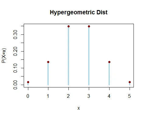
Graph of Hypergeometric Distribution H(5,5,20)

Following graph shows the probability mass function of hypergeometric distribution.

Key Features of Hypergeometric Distribution

• Suppose there are $N$ units in the population. These $N$ units are classified as $M$ successes and remaining $N-M$ failures.
• Out of $N$ units, $n$ units are selected at random without replacement.
• $X$ is the number of successes in the sample.

Mean of Hypergeometric Distribution

The expected value of hypergeometric randome variable is $E(X) =\dfrac{Mn}{N}$.

Proof

The expected value of hypergeometric randome variable is $$\begin{eqnarray*} % \nonumber to remove numbering (before each equation) E(x) &=& \sum_{x=0}^n x\frac{\binom{M}{x}\binom{N-M}{n-x}}{\binom{N}{n}}\\ &=& 0+ \sum_{x=1}^n x\frac{\frac{M!}{x!(M-x)!}\binom{N-M}{n-x}}{\frac{N!}{n!(N-n)!}}\\ &=& \sum_{x=1}^n \frac{\frac{M(M-1)!}{(x-1)!(M-x)!}\binom{N-M}{n-x}}{\frac{N(N-1)!}{n(n-1)!(N-n)!}}\\ &=& \frac{Mn}{N}\sum_{x=1}^n\frac{\binom{M-1}{x-1}\binom{N-M}{n-x}}{\binom{N-1}{n-1}} \end{eqnarray*}$$ Let $x-1=y$. So for $x=1$, $y=0$ and for $x=n$, $y=n-1$. Therefore $$\begin{eqnarray*} % \nonumber to remove numbering (before each equation) \mu_1^\prime &=& \frac{Mn}{N}\sum_{y=0}^{n-1}\frac{\binom{M-1}{y}\binom{N-M}{n-y-1}}{\binom{N-1}{n-1}} \\ &=& \frac{Mn}{N}\sum_{y=0}^{n^\prime}\frac{\binom{M-1}{y}\binom{N-M}{n^\prime-y}}{\binom{N-1}{n^\prime-1}} \\ &=&\frac{Mn}{N}\times 1. \end{eqnarray*}$$ Hence, mean = $E(X) =\dfrac{Mn}{N}$.

Variance of Hypergeometric Distribution

The variance of an hypergeometric random variable is $V(X) = \dfrac{Mn(N-M)(N-n)}{N^2(N-1)}$.

Proof

The variance of random variable $X$ is given by

$$\begin{equation*} V(X) = E(X^2) - [E(X)]^2. \end{equation*}$$

Let us find the expected value of $X(X-1)$.

$$\begin{eqnarray*} % \nonumber to remove numbering (before each equation) E[X(X-1)]&=& \sum_{x=0}^n x(x-1)\frac{\binom{M}{x}\binom{N-M}{n-x}}{\binom{N}{n}}\\ &=& 0+0+ \sum_{x=2}^n x\frac{\frac{M!}{x!(M-x)!}\binom{N-M}{n-x}}{\frac{N!}{n!(N-n)!}}\\ &=& \sum_{x=2}^n \frac{\frac{M(M-1)(M-2)!}{(x-2)!(M-x)!}\binom{N-M}{n-x}}{\frac{N(N-1)(N-2)!}{n(n-1)(n-2)!(N-n)!}}\\ &=& \frac{M(M-1)n(n-1)}{N(N-1)}\sum_{x=2}^n\frac{\binom{M-2}{x-2}\binom{N-M}{n-x}}{\binom{N-2}{n-2}} \end{eqnarray*}$$ Let $x-2=y$. So for $x=2$, $y=0$ and for $x=n$, $y=n-2$. Therefore $$\begin{eqnarray*} % \nonumber to remove numbering (before each equation) E[(X(X-1)]&=& \frac{Mn}{N}\sum_{y=0}^{n-2}\frac{\binom{M-2}{y}\binom{N-M}{n-y-2}}{\binom{N-2}{n-2}} \\ &=& \frac{Mn}{N}\sum_{y=0}^{n^\prime}\frac{\binom{M-2}{y}\binom{N-M}{n^\prime-y}}{\binom{N-2}{n^\prime}} \\ &=& \frac{M(M-1)n(n-1)}{N(N-1)}\times 1\\ & = &\frac{M(M-1)n(n-1)}{N(N-1)}. \end{eqnarray*}$$

$$\begin{eqnarray*} % \nonumber to remove numbering (before each equation) \mu_2^\prime &=& E[X(X-1)]+E(X) \\ &=& \frac{M(M-1)n(n-1)}{N(N-1)}+ \frac{Mn}{N}. \end{eqnarray*}$$ Hence, $$\begin{eqnarray*} % \nonumber to remove numbering (before each equation) \text{Variance = }\mu_2 &=& \mu_2^\prime -(\mu_1^\prime)^2 \\ &=& \frac{M(M-1)n(n-1)}{N(N-1)}+ \frac{Mn}{N}- \frac{M^2n^2}{N^2} \\ &=& \frac{Mn(N-M)(N-n)}{N^2(N-1)}. \end{eqnarray*}$$

Binomial as a limiting case of Hypergeometric distribution

In Hypergeometric distribution, if $N\to \infty$ and $\frac{M}{N}=p$, then the hypergeometric distribution tends to binomial distribution.

Proof

$$\begin{eqnarray*} % \nonumber to remove numbering (before each equation) P(X=x) &=& \lim_{N\to\infty} \frac{\binom{M}{x}\binom{N-M}{n-x}}{\binom{N}{n}}\\ &=& \lim_{N\to\infty} \frac{\bigg[\frac{M(M-1)\cdots (M-x+1)}{x!}\bigg]\bigg[\frac{(N-M)(N-M-1)\cdots (N-M-n+x+1)}{(n-x)!}\bigg]}{\frac{N(N-1)\cdots (N-n+1)}{n!}} \end{eqnarray*}$$ Dividing numerator and denominator by $N$, we get $$\begin{eqnarray*} & & P(X=x)\\ &=& \lim_{N\to\infty} \frac{n!}{x!(n-x)!}\frac{\frac{M}{N}(\frac{M}{N}-\frac{1}{N})\cdots (\frac{M}{N}-\frac{x-1}{N})(1-\frac{M}{N})(1-\frac{M}{N}-\frac{1}{N})\cdots (1-\frac{M}{N}-\frac{n-x-1}{N})}{1(1-\frac{1}{N})\cdots (1-\frac{n-1}{N})}\\ & = &\binom{n}{x}\frac{p(p-0)\cdots (p-0)(1-p)(1-p-0)\cdots (1-p-0)}{1(1-0)\cdots (1-0)}\;\;\; (\because \frac{M}{N}=p)\\ & = &\binom{n}{x}p^x (1-p)^{n-x}, x=0,1,2,\cdots, n; \; 0<p<1. \end{eqnarray*}$$ which is the probability mass function of binomial distribution.

Hope this tutorial helps you understand Hypergeometric distribution and various results related to Hypergeometric distributions.

Related Resources