Negative Binomial Distribution

Introduction

A negative binomial distribution is based on an experiment which satisfies the following three conditions:

• An experiment consists of q sequence of independent Bernoulli’s trials (i.e., each trial can result in a success ($S$) or a failure ($F$)),
• The probability of success is constant from trial to trial, i.e., $P(S\text{ on trial } i) = p$, for $i=1,2,3,\cdots$,
• The experiment continues until a total of $r$ successes have been observed, where $r$ is a specified positive integer.

Thus, a negative binomial experiment has the properties similar to Binomial distribution with the exception that the trials will be repeated until a fixed number of successes occur. If $X$ denote the number of failures that precede the $r^{th}$ success. then the random variable $X$ is called negative binomial random variable and the distribution of $X$ is called called negative binomial distribution.

Negative Binomial Distribution

Consider a sequence of independent repetitions of a Bernoulli’s trial with constant probability $p$ of success and $q$ of failure. Let the random variable $X$ denote the total number of failures in this sequence before the $r^{th}$ success, i.e., $X+r$ is equal to the number of trials necessary to produce exactly $r$ successes, where $r$ is a fixed positive integer. Here we are interested in finding the probability $x$ failures before $r^{th}$ success.

Number of ways of getting $(r-1)$ success out of $(x+r-1)$ trials equals $\binom{x+r-1}{r-1}$. Hence, probability of $x$ failures before $r$ successes is given by

$$ \begin{eqnarray*} P(X=x) &=& P[(r-1) \text{ success in } (x+r-1) \text{ trials }]\\ & & \quad \times P[r^{th} \text{ success in } (x+r) \text{ trials}] \\ &=& \binom{x+r-1}{r-1} p^{r-1} q^{x} \times p \\ &=& \binom{x+r-1}{r-1} p^{r} q^{x},\quad x=0,1,2,\ldots; r=1,2,\ldots\\ & & \qquad\qquad \qquad 0<p, q<1, p+q=1. \end{eqnarray*} $$

Definition of Negative Binomial Distribution

A discrete random variable $X$ is said to have negative binomial distribution if its p.m.f. is given by $$ \begin{eqnarray*} P(X=x)&=& \binom{x+r-1}{r-1} p^{r} q^{x},\quad x=0,1,2,\ldots; r=1,2,\ldots\\ & & \qquad\qquad \qquad 0<p, q<1, p+q=1. \end{eqnarray*} $$

Key Features of Negative Binomial Distribution

• A random experiment consists of repeated trials.
• Each trial of an experiment has two possible outcomes, like success ($S$) and failure ($F$).
• The probability of success ($p$) remains constants for each trial.
• The trials are independent of each other.
• The random variable is $X$ : the number of failures before getting $r^{th}$ success $(X = 0,1,2,\cdots )$.

Second form of Negative Binomial Distribution

Another form of negative binomial distribution can be obtained on simplifying $\binom{x+r-1}{r-1}$.

Consider $$ \begin{eqnarray*} \binom{x+r-1}{r-1} &=& \binom{x+r-1}{x} \\ &=& \frac{(x+r-1)(x+r-2)\cdots (r-1)r}{x!} \\ &=& \frac{(-1)^x (-r)(-r-1)\cdots(-r-x+2)(-r-x+1)}{x!}\\ & = & (-1)^x \binom{-r}{x}. \end{eqnarray*} $$

Thus, another form of p.m.f. of negative binomial distribution is $$ \begin{eqnarray*} P(X=x) &=& \binom{x+r-1}{r-1} p^{r} q^{x},\quad x=0,1,2,\ldots; r=1,2,\ldots\\ & & \qquad\qquad \qquad 0<p, q<1, p+q=1.\\ & = & (-1)^x \binom{-r}{x} p^r q^x \\ & = & \binom{-r}{x} p^r (-q)^x, \quad x=0,1,2,\ldots; r=1,2,\ldots\\ & & \qquad\qquad \qquad 0<p, q<1, p+q=1. \end{eqnarray*} $$

Third form of negative binomial distribution

Let $p = \dfrac{1}{Q}$ and $q=\dfrac{P}{Q}$. So $p+q =\dfrac{1}{Q}+\dfrac{P}{Q}= \dfrac{1+P}{Q}=1$. Hence we have $Q-P =1$.

Then the above p.m.f. can be written as $$ \begin{eqnarray*} P(X=x) & = & \binom{-r}{x} (1/Q)^r (-P/Q)^x, \quad x=0,1,2,\ldots\\ & & \qquad\qquad \qquad Q-P=1.\\ & = & \binom{-r}{x} Q^{-r} (-P/Q)^x, \quad x=0,1,2,\ldots\\ & & \qquad\qquad \qquad Q-P=1.\\ \end{eqnarray*} $$ $P(X=x)$ is $(x+1)^{th}$ terms in the expansion of $(Q-P)^{-r}$. It is known as negative binomial distribution because of $-$ve index.

Clearly, $P(x)\geq 0$ for all $x\geq 0$, and $$ \begin{eqnarray*} \sum_{x=0}^\infty P(X=x)&=& \sum_{x=0}^\infty \binom{-r}{x} Q^{-r} (-P/Q)^x, \\ &=& Q^{-r}\sum_{x=0}^\infty \binom{-r}{x} (-P/Q)^x, \\ &=& Q^{-r} \bigg(1-\frac{P}{Q}\bigg)^{-r}\;\quad \big(\because (1-q)^{-r} = \sum_{x=0}^\infty \binom{-r}{x} (-q)^x\big)\\ &=& Q^{-r} \bigg(\frac{Q-P}{Q}\bigg)^{-r}\\ &=& (Q-P)^{-r} = 1^{-r}=1. \end{eqnarray*} $$

Hence, $P(X=x)$ defined above is a legitimate probability mass function.

Geometric as a particular case of negative binomial

In negative binomial distribution, if $r=1$ then we get $$ \begin{equation*} P(X=x) = q^x p, x=0,1,2,\ldots,\;\; 0<p,q<1; p+q=1 \end{equation*} $$ which is the p.m.f. of geometric distribution. Hence Geometric distribution is the particular case of negative binomial distribution.

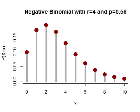
Graph of Negative Binomial Distribution

Following graph shows the probability mass function of negative binomial distribution with parameters $r=4$ and $p=0.56$.

Mean of Negative Binomial Distribution

The mean of negative binomial distribution is $E(X)=\dfrac{rq}{p}$.

Proof

The mean of random variable $X$ is given by $E(X)$.

$$ \begin{eqnarray*} \mu_1^\prime =E(X) &=& \sum_{x=0}^\infty x\cdot P(X=x) \\ &=& \sum_{x=0}^\infty x\cdot \binom{-r}{x} p^r (-q)^x\\ &=& p^r \sum_{x=0}^\infty x\frac{(-r)!}{x!(-r-x)!}\cdot (-q)^{x}\\ &=& p^r \sum_{x=1}^\infty \frac{(-r)(-r-1)!}{(x-1)!(-r-x)!}\cdot (-q)^{x}\\ &=& p^r(-r)(-q)\sum_{x=1}^\infty \binom{-r-1}{x-1}\cdot (-q)^{x-1}\\ &=& p^r rq\sum_{x=1}^\infty \binom{-r-1}{x-1}\cdot p^{r-1}(-q)^{x-1}\\ &=& p^rrq(1-q)^{-r-1}\\ &=& \frac{rq}{p}. \end{eqnarray*} $$

Variance of Negative Binomial Distribution

The variance of negative binomial distribution is $V(X)=\dfrac{rq}{p^2}$.

Proof

The variance of random variable $X$ is given by

$$ V(X) = E(X^2) - [E(X)]^2 $$

Let us find the expected value $X^2$. $$ \begin{eqnarray*} E(X^2) &=& E[X(X-1)+X] \\ &=& E[X(X-1)]+E(X)\\ &=& \sum_{x=0}^\infty x(x-1) P(X=x) +\frac{rq}{p}\\ &=& \sum_{x=0}^\infty \binom{-r}{x} p^r (-q)^x +\frac{rq}{p} \\ &=& p^r (-r)(-r-1)(-q)^2 \sum_{x=2}^\infty \binom{-r-2}{x-2}(-q)^{x-2}+\frac{rq}{p}\\ & =& r(r+1)q^2p^r (1-q)^{-r-2}+\frac{rq}{p}\\ &=& \frac{r(r+1)q^2p^r}{p^{r+2}}+\frac{rq}{p}\\ &=& \frac{r(r+1)q^2}{p^2}+\frac{rq}{p}. \end{eqnarray*} $$ Now, $$ \begin{eqnarray*} V(X) &=& E(X^2)-[E(X)]^2 \\ &=& \frac{r(r+1)q^2}{p^2}+\frac{rq}{p}-\frac{r^2q^2}{p^2}\\ &=& \frac{rq^2}{p^2}+\frac{rq}{p}\\ &=&\frac{rq}{p^2}. \end{eqnarray*} $$

For negative binomial distribution $V(X)> E(X)$, i.e., $\dfrac{rq}{p} > \dfrac{rq}{p^2}$.

MGF of Negative Binomial Distribution

The MGF of negative binomial distribution is $M_X(t)=\big(Q-Pe^{t}\big)^{-r}$.

Proof

The MGF of negative binomial distribution is

$$ \begin{eqnarray*} M_X(t) &=& E(e^{tX}) \\ &=& \sum_{x=0}^\infty e^{tx} \binom{-r}{x} Q^{-r} (-P/Q)^x, \\ &=& \sum_{x=0}^\infty \binom{-r}{x} Q^{-r} (-Pe^{t}/Q)^x, \\ &=& Q^{-r} \bigg(1-\frac{Pe^{t}}{Q}\bigg)^{-r}\\ &=& Q^{-r} \bigg(\frac{Q-Pe^{t}}{Q}\bigg)^{-r}\\ &=& \big(Q-Pe^{t}\big)^{-r}. \end{eqnarray*} $$

Hence, the m.g.f. of negative binomial distribution is $M_X(t)=\big(Q-Pe^{t}\big)^{-r}$.

Mean and Variance Using MGF

$$ \begin{eqnarray*} \mu_1^\prime &=& \bigg[\frac{d}{dt} M_X(t)\bigg]_{t=0}\\ &=& \bigg[\frac{d}{dt} (Q-Pe^t)^{-r}\bigg]_{t=0} \\ &=& \big[(-r)(Q-Pe^t)^{-r-1} Pe^t (-1)\big]_{t=0}\\ & = & rP\big[(Q-Pe^t)^{-r-1}e^t\big]_{t=0}\\ & = & rP\qquad (\because Q-P =1). \end{eqnarray*} $$

$$ \begin{eqnarray*} \mu_2^\prime &=& \bigg[\frac{d^2}{dt^2} M_X(t)\bigg]_{t=0}\\ &=&\bigg[\frac{d}{dt} rPe^t(Q-Pe^t)^{-r-1}\bigg]_{t=0} \\ &=& rP\bigg[e^t(-r-1)(Q-Pe^t)^{-r-2}(-Pe^t)+(Q-Pe^t)^{-r-1}e^t\bigg]_{t=0} \\ &=& rP\bigg[ (r+1)Pe^{2t}(Q-Pe^t)^{-r-2}+(Q-Pe^t)^{-r-1}e^t\bigg]_{t=0}\\ &=& r(r+1)P^2 +rP. \end{eqnarray*} $$ Therefore, $$ \begin{eqnarray*} \mu_2 &=& \mu_2^\prime-(\mu_1^\prime)^2 \\ &=& r(r+1)P^2 +rP-(rP)^2\\ &=& r^2P^2 + rP^2+rP - r^2P^2\\ & = & rP(P+1)\\ &=& rPQ. \end{eqnarray*} $$

Hence, mean $= \mu_1^\prime =rP$ and variance $=\mu_2 = rPQ$.

The MGF of negative binomial distribution is $M_X(t)=\big(Q-Pe^{t}\big)^{-r}$.

Letting $p=\dfrac{1}{Q}$ and $q=\dfrac{P}{Q}$, the m.g.f. of negative binomial distribution in terms of $p$ and $q$ is $M_X(t) =p^r(1-qe^t)^{-r}$.

In terms of $p$ and $q$, the mean and variance of negative binomial distribution are respectively $\dfrac{rq}{p}$ and $\dfrac{rq}{p^2}$.

CGF of Negative Binomial Distribution

The CGF of negative binomial distribution is $K_X(t)=-r\log_e(Q-Pe^t)$.

Proof

The CGF of negative binomial distribution is $$ \begin{eqnarray*} K_X(t) &=& \log_e M_X(t)\\ &=& -r\log_e(Q-Pe^t). \end{eqnarray*} $$

$$ \begin{eqnarray*} K_X(t)&=& -r\log_e(Q-Pe^t)\\ &=& -r\log_e\bigg[Q-P\bigg(1+t +\frac{t^2}{2!}+ \frac{t^3}{3!}+\cdots \bigg) \bigg]\\ &=& -r\log_e\bigg[Q-P-P\bigg(t +\frac{t^2}{2!}+ \frac{t^3}{3!}+\cdots \bigg) \bigg]\\ &=& -r\log_e\bigg[1-P\bigg(t +\frac{t^2}{2!}+ \frac{t^3}{3!}+\cdots \bigg) \bigg]\\ &=& r\bigg[P\bigg(t +\frac{t^2}{2!}+ \frac{t^3}{3!}+\cdots \bigg)+\frac{P^2}{2}\bigg(t +\frac{t^2}{2!}+ \frac{t^3}{3!}+\cdots \bigg)^2+\\ & &\frac{P^3}{3}\bigg(t +\frac{t^2}{2!}+ \frac{t^3}{3!}+\cdots \bigg)^3+\frac{P^4}{4}\bigg(t +\frac{t^2}{2!}+ \frac{t^3}{3!}+\cdots \bigg)^4+\cdots \bigg] \end{eqnarray*} $$

The $r^{th}$ cumulant of $X$ is given by

$$ \begin{equation*} \kappa_r = \text{coefficient of $\frac{t^r}{r!}$ in the expansion of $K_X(t)$} \end{equation*} $$

Collecting the coefficient of $\frac{t^r}{r!}$ from the expansion of $K_X(t)$, we have

$$ \begin{eqnarray*} \kappa_1 =\mu_1^\prime &=& \text{coefficient of $t$ in the expansion of $K_X(t)$} \\ &=& rP \\ \end{eqnarray*} $$

$$ \begin{eqnarray*} \kappa_2 =\mu_2 &=& \text{coefficient of $\frac{t^2}{2!}$ in the expansion of $K_X(t)$} \\ &=& r(P+P^2) \\ & = & rP(1+P) = rPQ. \end{eqnarray*} $$

$$ \begin{eqnarray*} \kappa_3 =\mu_3 &=& \text{coefficient of $\frac{t^3}{3!}$ in the expansion of $K_X(t)$} \\ &=& r(P+3P^2+2P^3) \\ &=& rP(1+3P+2P^2)\\ &=& rP(1+P)(1+2P). \end{eqnarray*} $$

$$ \begin{eqnarray*} \kappa_4 &=& \text{coefficient of $\frac{t^4}{4!}$ in the expansion of $K_X(t)$} \\ &=& r[P+(3P^2+4P^2) + (6P^3+6P^3) + 6P^4] \\ &=& rPQ(1+6PQ) \end{eqnarray*} $$

Hence, $$ \begin{eqnarray*} \mu_4 &=& \kappa_4 + 3\kappa_2^2 \\ &=& rPQ [1+3PQ(r+2)]. \end{eqnarray*} $$

Characteristics Function of negative binomial distribution

The characteristics function of negative binomial distribution is

$\phi_X(t) = p^r (1-qe^{it})^{-r}$.

Proof

The characteristics function of negative binomial distribution is $$ \begin{eqnarray*} \phi_X(t) &=& E(e^{itX})\\ &=& M_X(it) \\ &=& (Q-Pe^{it})^{-r}\\ &=& p^r (1-qe^{it})^{-r}. \end{eqnarray*} $$

Recurrence Relation for the probability of Negative Binomial Distribution

The recurrence relation for the probabilities of negative binomial distribution is

$$ \begin{equation*} P(X=x+1) = \frac{(x+r)}{(x+1)} q \cdot P(X=x),\quad x=0,1,\cdots \end{equation*} $$ where $P(X=0) = p^r$.

Proof

The p.m.f. of negative binomial distribution is $$ \begin{equation*} P(X=x) = \binom{x+r-1}{r-1} p^{r} q^{x} \end{equation*} $$ Then $P(X=x+1)$ is $$ \begin{aligned} P(X=x+1) &= \binom{x+1+r-1}{r-1} p^{r} q^{x+1}\\ &=\binom{x+r}{r-1} p^{r} q^{x+1} \end{aligned} $$

Taking the ratio of $P(X=x+1)$ and $P(X=x)$, we have $$ \begin{eqnarray*} \frac{P(X=x+1)}{P(X=x)} &=& \frac{\binom{x+r}{r-1} p^{r} q^{x+1}}{\binom{x+r-1}{r-1} p^{r} q^{x}} \\ &=& \frac{(x+r)!}{(r-1)!(x+1)!}\frac{(r-1)!x!}{(x+r-1)!}q \\ &=& \frac{(x+r)}{(x+1)}q. \end{eqnarray*} $$ Hence, the recurrence relation for probabilities of negative binomial distribution is $$ \begin{equation*} P(X=x+1) = \frac{(x+r)}{(x+1)} q \cdot P(X=x),\quad x=0,1,\cdots \end{equation*} $$ where $P(X=0) = p^r$.

Poisson Distribution as a limiting case of Negative Binomial Distribution

Negative binomial distribution $NB(r, p)$ tends to Poisson distribution as $r\to \infty$ and $P\to 0$ with $rP = \lambda$ (finite).

Proof

Let $X\sim NB(r,P)$ distribution.

Then the PMF of $X$ is

$$ \begin{equation*} P(X=x) =\binom{x+r-1}{r-1} Q^{-r}(P/Q)^x. \end{equation*} $$

$$ \begin{eqnarray*} \lim_{r\to \infty \atop P\to 0} P(X=x) &=& \lim_{r\to \infty\atop P\to 0} \binom{x+r-1}{r-1} Q^{-r}(P/Q)^x \\ &=& \lim_{r\to \infty \atop P\to 0} \frac{(x+r-1)!}{x!(r-1)!} (1+P)^{-r}\bigg(\frac{P}{1+P}\bigg)^x \\ &=& \lim_{r\to \infty\atop P\to 0} \frac{(x+r-1)(x+r-2)\cdots (r+1)\cdot r}{x!} (1+P)^{-r}\bigg(\frac{P}{1+P}\bigg)^x \\ &=& \lim_{r\to \infty\atop P\to 0} \frac{r^x}{x!}\cdot\frac{(x+r-1)}{r}\cdot \frac{(x+r-2)}{r}\cdots \frac{(r+1)}{r}\cdot \frac{r}{r} (1+P)^{-r}\bigg(\frac{P}{1+P}\bigg)^x\\ &=& \lim_{r\to \infty\atop P\to 0} \frac{(rP)^x}{x!}\cdot\bigg(1+\frac{x-1}{r}\bigg)\cdot \bigg(1+\frac{x-2}{r}\bigg)\cdots \bigg(1+\frac{1}{r}\bigg) (1+P)^{-r}(1+P)^{-x}\\ &=& \frac{\lambda^x}{x!}\lim_{r\to \infty\atop P\to 0} \bigg(1+\frac{x-1}{r}\bigg)\cdot \bigg(1+\frac{x-2}{r}\bigg)\cdots \bigg(1+\frac{1}{r}\bigg) (1+P)^{-r}(1+P)^{-x}\\ &=& \frac{\lambda^x}{x!}\lim_{r\to \infty} \bigg(1+\frac{\lambda}{r}\bigg)^{-r}\lim_{r\to \infty}\bigg(1+\frac{\lambda}{r}\bigg)^{-x}, \quad (\because \lambda = rP) \end{eqnarray*} $$ But $$ \begin{equation*} \lim_{r\to \infty}\bigg(1+\frac{\lambda}{r}\bigg)^{-x}=1, \text{ and } \lim_{r\to \infty}\bigg(1+\frac{\lambda}{r}\bigg)^{-r}=e^{-\lambda}. \end{equation*} $$ Hence, $$ \begin{eqnarray*} \lim_{r\to \infty, P\to 0} P(X=x) &=& \frac{e^{-\lambda}\lambda^x}{x!}, \quad x=0,1,2,\cdots,\; \; \lambda>0 \end{eqnarray*} $$ which is the probability mass function of Poisson distribution.

Related Resources